【R语言】如何进行英文分词统计（以《爱丽丝漫游奇境》词频统计为例)（20年3月22日复习笔记）

老师所给的题目要求是

这是一道对英文进行分词的词频统计。
首先当然是要导入这个文档以及所需要的的包（绘制频数图需要ggplot2包，绘制词云需要wordcloud2包）

###################################################
setwd("D://1Study//R//CH 03") 
getwd()
###################################################
library(ggplot2)
library(wordcloud2) #绘制词云的包

其中，老师介绍了两种导入文档的方式，一种是全文读入，一种是逐行读入。先说全文读入的方法

一、全文读入

#法一：全文本读入，用scan扫描文件
txt = scan("Alice's Adventures in Wonderland - Lewis Carroll.txt","")
#用意同↓，以字符串格式读入txt
#txt = scan("Alice's Adventures in Wonderland - Lewis Carroll.txt",what = "c")
txt

关于scan读入文档的语句，翔宇亭IT乐园前辈介绍了scan语法的五种例句:

（1）scan(“student.txt”, what=“c”) #以字符串的格式读取数据
（2）scan(“student.txt”, what=“c”, nlines=3) #读取3行
（3）scan(“student.txt”, what=“c”, skip=1) #忽略第1行
（4）scan(“student.txt”, what = list(studentNo="", studentName="", studentSex="", studentAge=0), skip=1) #以列表的形式读取数据
（5）lst <- scan(“student.txt”, what = list(xh="", xm="", xb="", nl=0), skip=1) #读取数据并保存到变量中

运行结果如图

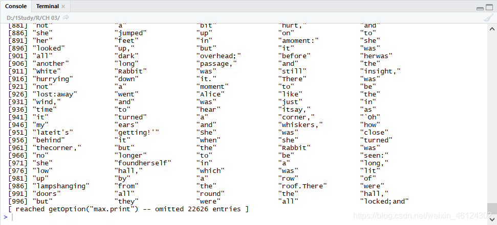
我们发现，运行结果存在两个问题
1.标点符号也会被作为单词的一部分读入，因为txt = scan(“Alice’s Adventures in Wonderland - Lewis Carroll.txt”,"")以字符串读入，仅以“空格”作为分隔单词和单词的手段。
2.未区分大小写，There和there会被算作两个不同的词。
需要对数据进行再处理。

所以老师建议采用逐行读入，逐行处理的方式。也就是下文将介绍的方法

二、逐行读入并处理

逐行读取法有以下几点需要注意

1.readLines函数的使用

我们可以发现，这里用的是readLines函数，con表示

a connection object or a character string.

也就是要逐行处理的对象，n等于的值表示

integer. The (maximal) number of lines to read. Negative values indicate that one should read up to the end of input on the connection.
整数。要读取的（最大）行数。负值表示应该读取到连接上输入的末尾。

#法二：逐行读取，并在读取过程中逐行处理异常文本
con = file("Alice's Adventures in Wonderland - Lewis Carroll.txt","r")
#定义一个变量用于读取文件

line = readLines(con,n = 1)
#读取con的第一行

这里的readLines函数的使用含义是，读取con的第一行

2.循环语句

while (length(line)!=0) {

这个循环语句起到了两个效果
(1)异常处理
确保文章内容非空
(2)没有终结点
确保文章读完，一直往下做循环。我们可以用如下语句测试一下

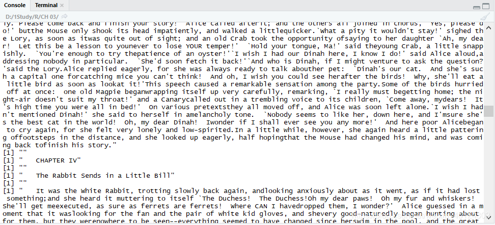
#接下来开始做循环，从第一行往下循环
while (length(line)!=0) {#确保不是空的文章，异常处理;逐行处理
  print(line)
  line = readLines(con,n = 1)
}

运行结果如图

不过对于这一语句，我存在如下疑问

help里说这个函数的n起到的是最大值的作用，最大读到第n行，如果要全部读完需要赋值为负
我比较好奇的是，为什么这个语句里没有n++的描述，但是还是能读完全部文章，而不是疯狂读第一句话呢

这里我先挖个坑，等我整明白了再回来补充

3.大小写处理

这个比较简单

temp_line = tolower(line) #全部转化为小写

即可

4.特殊字符处理

有两种方式处理
(1)使用gsub函数对特殊符号一个一个替换

  temp_line = gsub("'s"," is ", temp_line)#把temp_line中的s转化成is
  temp_line = gsub("'s"," is ", temp_line)
  temp_line = gsub(";"," ", temp_line)
  temp_line = gsub(","," ", temp_line)
  temp_line = gsub("'"," ", temp_line)
  temp_line = gsub(":"," ", temp_line)
  temp_line = gsub("-"," ", temp_line)
  temp_line = gsub("`"," ", temp_line)
  temp_line = gsub("\n"," ", temp_line)
  temp_line = gsub('\"'," ", temp_line, fixed = TRUE)
  temp_line = gsub("?"," ", temp_line, fixed = TRUE)
  temp_line = gsub("*"," ", temp_line, fixed = TRUE)
  temp_line = gsub("."," ", temp_line, fixed = TRUE)
  #要用fixed是因为
  #通配符(用于匹配特定字符的符号<如.匹配全部字母>，这里就把.？\*等字符，默认转化为通配符。
  #为了避免使用通配符，必须修复

注意，像.？*等字符是通配符，也就是说代表着一些字母或符号，比如"."就是代表全部字母，直接替换会把他们代表的东西全替换了，所以要在fixed属性中设为TRUE

fixed
logical. If TRUE, pattern is a string to be matched as is. Overrides all conflicting arguments.

(2)正则表达式

temp_line = gsub("[^a-zA-Z]"," ",temp_line)     #正则表达式

表示匹配所有非字母字符
更多正则表达式的匹配，在gearss前辈的博文中有详细的归纳。

5.保存文件

#保存文件，以方便未来使用
out_con = file("processTXT20200322.txt","w")#用w写模式写入保存(这种模式下可以修改文件)
write(processed,out_con,ap

6.提取词频

# 重新提取每一个处理好的词
composition = strsplit(x = processsed,split = " ")# 按照空格拆分文本为一个一个的词

！注意：这种方法只在英文下生效，中文没有空格，我们必须使用中文分词法

7.建立词频表

建立表格

wordsFreq = data.frame(table(composition))
wordsFreq[,1] = as.character(wordsFreq[,1])#为方便后续操作，把第一行的单词转换为字符型

建立完表格后，我们会发现，表格中出现了空格和一些没有含义的词

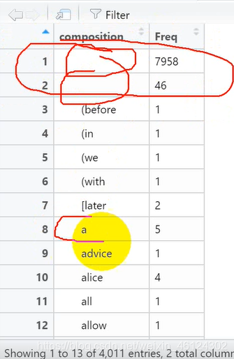
所以我们**用“当单词的长度小于2时，删除该单词”的方法过滤上述词频 **

wordsFreq = wordsFreq[-which(nchar(wordsFreq[,1])<2),]  #当单词的长度小于2时，删除该单词

-表示排除，which指定内容，nchar指代“某个字符串的长度”

当然，我们也可以顺便过滤一下最低词频，只出现一次的词我们也不留

wordsFreq = wordsFreq[which(wordsFreq[,2]>2),] 

因为我们要找的是前50个频繁词，所以要排一下顺序（前500个同理）

wordsFreq = wordsFreq[order(-wordsFreq$Freq),]#从大到小排序

然后保留前50个

wordsFreq[1:50,]
data = wordsFreq[1:50,]#取前50个保存

至此，数据处理的部分就完成了。

三、画图

1.柱状图

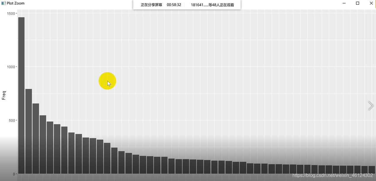
ggplot(data = data, aes(x=composition,y=Freq))+geom_bar(stat = "identity")#属性指代XY轴名字和类型(柱状图)

结果如图

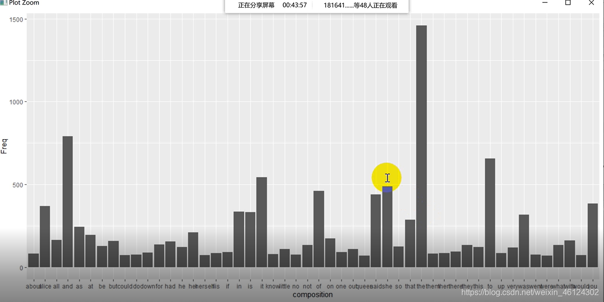
# 修改词语纵向排列
ggplot(data = data, aes(x=composition,y=Freq))+geom_bar(stat = "identity")+theme(axis.text.x = element_text(angle = 90,hjust = 1))    #angle表示角度，hjust表示距离

X轴的文字都挤在一块儿了，可以改成纵向排列的↑
当然，为了再美观一点，我们也可以再作图使其从大到小排列↓

# 设置柱状条形图的顺序
data$composition = factor(data$composition,levels = c(data$composition))  #设置柱状条形图的顺序
ggplot(data = data, aes(x=composition,y=Freq))+geom_bar(stat = "identity")+theme(axis.text.x = element_text(angle = 90,hjust = 1)) 

2.词云

#词云
data = wordsFreq[1:300,]
wordcloud2(data,size = 1)
wordcloud2(data,size = 1,shape = "star")

补充：如何使用停止词文档

如果有专门的停止词txt的话，也可以加以使用，过滤到诸如"he""she"等无意义词

# 停用词问题
# tm包里面内置的一部分停用词
stopwords = read.table("stopwords.txt",header = FALSE)
clean_wordsFreq = wordsFreq
for (word in wordsFreq$composition){
  if (word %in% stopwords$V1){
    clean_wordsFreq = clean_wordsFreq[-which(clean_wordsFreq[,1]==word),]
  }
}
data = clean_wordsFreq[1:50,]

最后附上完整代码

###################################################
setwd("D://1Study//R//CH 03") 
getwd()
###################################################
library(ggplot2)
#library(NLP)  #自然语言处理的包
#library(tm)   #文本挖掘的包
library(wordcloud2) #绘制词云的包

#####
#1.读取小说
#法一：全文本读入，用scan扫描文件
txt = scan("Alice's Adventures in Wonderland - Lewis Carroll.txt","")
#用意同↓，以字符串格式读入txt
#txt = scan("Alice's Adventures in Wonderland - Lewis Carroll.txt",what = "c")
txt
#法一不太好，因为标点符号也会被作为单词读入

#法二：逐行读取，并在读取过程中逐行处理异常文本
processed = ""#用来保存文本

con = file("Alice's Adventures in Wonderland - Lewis Carroll.txt","r")
#定义一个变量用于读取文件

line = readLines(con,n = 1)
#读取con的第一行

#接下来开始做循环，从第一行往下循环
while (length(line)!=0) {#确保不是空的文章，异常处理;逐行处理
  temp_line = tolower(line) #全部转化为小写
  temp_line = gsub("'s"," is ", temp_line)#把temp_line中的s转化成is
  temp_line = gsub("'s"," is ", temp_line)
  temp_line = gsub(";"," ", temp_line)
  temp_line = gsub(","," ", temp_line)
  temp_line = gsub("'"," ", temp_line)
  temp_line = gsub(":"," ", temp_line)
  temp_line = gsub("-"," ", temp_line)
  temp_line = gsub("`"," ", temp_line)
  temp_line = gsub("\n"," ", temp_line)
  temp_line = gsub('\"'," ", temp_line, fixed = TRUE)
  temp_line = gsub("?"," ", temp_line, fixed = TRUE)
  temp_line = gsub("*"," ", temp_line, fixed = TRUE)
  temp_line = gsub("."," ", temp_line, fixed = TRUE)
  #要用fixed是因为
  #通配符(用于匹配特定字符的符号<如.匹配全部字母>，这里就把.？\*等字符，默认转化为通配符。
  #为了避免使用通配符，必须修复
  
  processed = paste(processed,temp_line," ")#连接已有内容和新加入行的内容,中间用空格分开
  #即↓
  #processed = paste(processed,temp_line,sep = " ")
  processed
  line = readLines(con,n = 1)
}

#####
#保存文件，以方便未来使用
out_con = file("processTXT20200322.txt","w")#用w写模式写入保存(这种模式下可以修改文件)
write(processed,out_con,append = TRUE)#append表示允许追加
close(out_con)#关闭文件
getwd()


######
# 重新提取每一个处理好的词
composition = strsplit(x = processsed,split = " ")# 按照空格拆分文本为一个一个的词
#！注意：这种方法只在英文下生效，中文没有空格，我们必须使用中文分词法

# 建立频数表
wordsFreq = data.frame(table(composition))
wordsFreq[,1] = as.character(wordsFreq[,1])#为方便后续操作，把第一行的单词转换为字符型

wordsFreq = wordsFreq[-which(nchar(wordsFreq[,1])<2),]  #当单词的长度小于2时，删除该单词

wordsFreq = wordsFreq[order(-wordsFreq$Freq),]#从大到小排序

wordsFreq[1:50,]
data = wordsFreq[1:50,]#取前50个保存

#####
#画图

#柱状图
#属性指代XY轴名字和类型(柱状图)
data$composition = factor(data$composition,levels = c(data$composition))  #设置柱状条形图的顺序
ggplot(data = data, aes(x=composition,y=Freq))+geom_bar(stat = "identity")+theme(axis.text.x = element_text(angle = 90,hjust = 1)) 

#词云
data = wordsFreq[1:300,]
wordcloud2(data,size = 1)
wordcloud2(data,size = 1,shape = "star")

######
# 注:tm包里面内置的一部分停用词
stopwords = read.table("stopwords.txt",header = FALSE)
clean_wordsFreq = wordsFreq
for (word in wordsFreq$composition){
  if (word %in% stopwords$V1){
    clean_wordsFreq = clean_wordsFreq[-which(clean_wordsFreq[,1]==word),]
  }
}
data = clean_wordsFreq[1:50,]

以上是我对英文分词词频统计的理解，如果表述有误，欢迎批评指正。