绪论

在训练神经网络模型的时候，当模型训练完之后，确切地说当训练的session关闭之后，我们训练出来的模型参数会全部丢失，从而无法有效复用模型，而TensorFlow中提供了很好地保存模型和提取模型的方法。

1. Tensorflow的模型到底是什么样的？

Tensorflow模型主要包含网络的设计（图）和训练好的各参数的值等。所以，Tensorflow模型有四个文件：
在这里插入图片描述

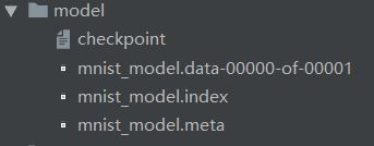
① checkpoint 文件会记录保存信息，通过它可以定位最新保存的模型
② model.ckpt.data-xxx 文件保存了当前参数值
③ model.ckpt.index 文件保存了当前参数名
④ model.ckpt.meta 文件保存了Tensorflow图；即所有的变量、操作、集合等

2. Tensorflow模型的保存

① 首先，为了保存Tensorflow中的图和所有参数的值，我们创建一个tf.train.Saver()类的实例。

saver = tf.train.Saver()

② 由于Tensorflow变量仅存在于session内，所以必须在session内进行保存，可通过调用创建的saver对象的save方法实现。

saver.save(sess, path+"model_conv/my-model", global_step=epoch)

其中：

sess是session对象。
path+"model_conv/my-model"是你对自己模型的路径+命名。
global_step表示迭代多少次就保存模型（比如每迭代1000次后保存模型：global_step=1000），一般使用全局步数global_step，这样才能够实现断点继训。
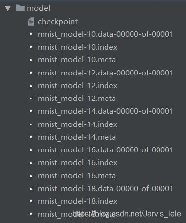
如果你想保存最近的4个模型并且每训练两个小时保存一次，可以使用 max_to_keep=4 和 keep_checkpoint_every_n_hours=2。
Tensorflow中默认保存最近的5个模型。

③ 我们在tf.train.Saver()中并没有指定任何东西，因此它将保存所有变量。如果我们不想保存所有的变量，只想保存其中一些变量，我们可以在创建tf.train.Saver实例的时候，给它传递一个我们想要保存的变量的list或者字典。示例如下：

import tensorflow as tf
w1 = tf.Variable(tf.random_normal(shape=[2]), name='w1')
w2 = tf.Variable(tf.random_normal(shape=[5]), name='w2')
saver = tf.train.Saver([w1,w2])
sess = tf.Session()
sess.run(tf.global_variables_initializer())
saver.save(sess, 'my_test_model',global_step=1000)

实例代码：

import tensorflow as tf

#Prepare to feed input, i.e. feed_dict and placeholders
w1 = tf.placeholder("float", name="w1")
w2 = tf.placeholder("float", name="w2")
b1= tf.Variable(2.0,name="bias")


#Define a test operation that we will restore
w3 = tf.add(w1,w2)
w4 = tf.multiply(w3,b1,name="op_to_restore")
with tf.Session() as sess:
	sess.run(tf.global_variables_initializer())
	
	#Create a saver object which will save all the variables
	saver = tf.train.Saver()
	
	#Run the operation by feeding input
	print(sess.run(w4,feed_dict ={w1:4,w2:8}))
	#Prints 24 which is sum of (w1+w2)*b1
	
	#Now, save the graph
	saver.save(sess, './my_test_model',global_step=1000)

3.Tensorflow模型的加载

如果要使用已经训练好的模型，那么你需要做两个步骤：

① 创建网络Create the network:

你可以通过写python代码，来手动地创建每一个、每一层，使得跟原始网络一样。

但是，如果你仔细想的话，我们已经将模型保存在了 .meta 文件中，因此我们可以使用tf.train.import()函数来重新创建网络，使用方法如下：

saver = tf.train.import_meta_graph('./my_test_model-1000.meta')

注意，这仅仅是将已经定义的网络导入到当前的graph中，但是我们还是需要加载网络的参数值。

② 加载参数Load the parameters

我们可以通过调用restore函数来恢复网络的参数，如下：

with tf.Session() as sess:
  new_saver = tf.train.import_meta_graph('my_test_model-1000.meta')
  new_saver.restore(sess, tf.train.latest_checkpoint('./'))

在这之后，像w1和w2的tensor的值已经被恢复，并且可以获取到：

with tf.Session() as sess:    
    saver = tf.train.import_meta_graph('my-model-1000.meta')
    saver.restore(sess,tf.train.latest_checkpoint('./'))
    print(sess.run('w1:0'))
##Model has been restored. Above statement will print the saved value of w1.

实例代码：

  上面介绍了如何保存和恢复一个Tensorflow模型。下面介绍一个加载任何预训练模型的实用方法。
  现在，我们想要恢复这个网络，我们不仅需要恢复图（graph）和权重，而且也需要准备一个新的
  feed_dict，将新的训练数据喂给网络。

我们可以通过使用graph.get_tensor_by_name()方法来获得已经保存的操作（operations）和placeholder variables。

#How to access saved variable/Tensor/placeholders 
graph = tf.get_default_graph()
w1 = graph.get_tensor_by_name("w1:0")
## How to access saved operation
op_to_restore = graph.get_tensor_by_name("op_to_restore:0")

（注：

操作的名称为训练模型中name后面的名称
如果参数是这样保存的：

 with tf.name_scope('conv1'):
    W1 = tf.Variable(tf.truncated_normal([784, 500], stddev=0.1), name='W1')

那么调用的时候需注意：

graph = tf.get_default_graph()
w1 = graph.get_tensor_by_name("conv1/w1:0")

如果我们仅仅想要用不同的数据运行这个网络，可以简单的使用feed_dict来将新的数据传递给网络。

import tensorflow as tf

with tf.Session() as sess:
    #First let's load meta graph and restore weights
    saver = tf.train.import_meta_graph('./my_test_model-1000.meta')
    saver.restore(sess,tf.train.latest_checkpoint('./'))


    # Now, let's access and create placeholders variables and
    # create feed-dict to feed new data

    graph = tf.get_default_graph()
    w1 = graph.get_tensor_by_name("w1:0")
    w2 = graph.get_tensor_by_name("w2:0")


    #Now, access the op that you want to run.
    op_to_restore = graph.get_tensor_by_name("op_to_restore:0")
    '''
	#Add more to the current graph
	add_on_op = tf.multiply(op_to_restore,2)
	
	print sess.run(add_on_op,feed_dict ={w1:13.0,w2:17.0})
	#This will print 120.
	'''
    print (sess.run(op_to_restore,feed_dict ={w1:13.0,w2:17.0}))

4. 如何保存pb文件和读取pb文件

上面模型的保存文件为ckpt文件，有多个文件组成。但很多时候，我们需要将TensorFlow的模型导出为单个文件（同时包含模型结构的定义与权重），方便在其他地方使用（如在Android中部署网络）。

下面的代码展示了最简单的tensorflow四则运算计算图：

 import tensorflow as tf

x = tf.placeholder(tf.float32,name="input")

a = tf.Variable(tf.constant(5.,shape=[1]),name="a")
b = tf.Variable(tf.constant(6.,shape=[1]),name="b")
c = tf.Variable(tf.constant(10.,shape=[1]),name="c")
d = tf.Variable(tf.constant(2.,shape=[1]),name="d")

tensor1 = tf.multiply(a,b,"mul")
tensor2 = tf.subtract(tensor1,c,"sub")
tensor3 = tf.div(tensor2,d,"div")
result = tf.add(tensor3,x,"add")

inial = tf.global_variables_initializer()
with tf.Session() as sess:
    sess.run(inial)
    print(sess.run(a))
    print(result)
    result = sess.run(result,feed_dict={x:1.0})
    print(result)
    constant_graph = tf.graph_util.convert_variables_to_constants(sess, sess.graph_def, ["add"])
    with tf.gfile.FastGFile("wsj.pb", mode='wb') as f:
        f.write(constant_graph.SerializeToString())

保存pb文件的功能主要是通过下面三行代码实现的

constant_graph = tf.graph_util.convert_variables_to_constants(sess, sess.graph_def, ["add"])
with tf.gfile.FastGFile("wsj.pb", mode='wb') as f:
    f.write(constant_graph.SerializeToString())

第一行代码的作用是将计算图中的变量转化为常量，并指定输出节点为“add”
第二行代码用来生成一个名为wsj.pb的文件（未指定路径的话，默认在该python代码的同路径下生成）
第三行代码的作用是将计算图写入该pb文件中

读取pb文件

import tensorflow as tf

with tf.gfile.FastGFile("wsj.pb", "rb") as f:
    graph_def = tf.GraphDef()
    graph_def.ParseFromString(f.read())
    result, x = tf.import_graph_def(graph_def,return_elements=["add:0", "input:0"])

with tf.Session() as sess:
    init = tf.global_variables_initializer()
    sess.run(init)
    print(sess.run(a))
    result = sess.run(result, feed_dict={x: 5.0})
    print(result)

上面代码主要分为两部分：读取pb文件并设置为默认的计算图；填充一个新的x值来计算结果。

读取pb文件时候需要注意的是，若要获取对应的张量必须用“tensor_name:0”的形式，这是tensorflow默认的。

5. 断点继训

顾名思义，断点续训的意思是因为某些原因模型还没有训练完成就被中断，下一次训练可以在上一次训练的基础上继续训练而不用从头开始；这种方式对于你那些训练时间很长的模型来说非常友好。

如果要进行断点续训，那么得满足两个条件：

（1）本地保存了模型训练中的快照；（即断点数据保存）

（2）可以通过读取快照恢复模型训练的现场环境。（断点数据恢复）

这两个操作都用到了tensorflow中的train.Saver类。
具体代码如下：

 ckpt = tf.train.get_checkpoint_state(MODEL_SAVE_PATH)
    if ckpt and ckpt.model_checkpoint_path:
        saver.restore(sess, ckpt.model_checkpoint_path)
  ······
  saver.save(sess, os.path.join(MODEL_SAVE_PATH, MODEL_NAME), global_step=global_step)
  #global_step为全局步数

6. 如何使用预训练好的模型来用于Finetuning

Finetuning的意思是在已有模型之后进行参数和训练模型复用的缩写，也是真实工程应用中最常用的的是由既有模型的手段。
我们可以通过graph.get_tensor_by_name() 方法来获取合适的operation，然后在这上面建立graph。下面是一个实际的例子，我们使用meta graph 加载了一个预训练好的vgg模型，并且在最后一层将输出个数改成2，然后用新的数据Finetuning。

......
......
saver = tf.train.import_meta_graph('vgg.meta')
# Access the graph
graph = tf.get_default_graph()
## Prepare the feed_dict for feeding data for fine-tuning 

#Access the appropriate output for fine-tuning
fc7= graph.get_tensor_by_name('fc7:0')

#use this if you only want to change gradients of the last layer
fc7 = tf.stop_gradient(fc7) # It's an identity function
fc7_shape= fc7.get_shape().as_list()

new_outputs=2
weights = tf.Variable(tf.truncated_normal([fc7_shape[3], num_outputs], stddev=0.05))
biases = tf.Variable(tf.constant(0.05, shape=[num_outputs]))
output = tf.matmul(fc7, weights) + biases
pred = tf.nn.softmax(output)

# Now, you run this with fine-tuning data in sess.run()

完整代码

最后，只需要在我们前面所写好的mnist代码中加入上面的语句，即可保存和恢复我们训练好的模型了，完整代码如下：

MNIST_TRAIN.py

import tensorflow as tf
import os
from tensorflow.examples.tutorials.mnist import input_data

mnist = input_data.read_data_sets("MNIST_data", one_hot=True)

'''
定义固定的超参数,方便待使用时直接传入。如果你问，这个超参数为啥要这样设定，如何选择最优的超参数？
这个问题此处先不讨论，超参数的选择在机器学习建模中最常用的方法就是“交叉验证法”。
另外，还要设置两个路径，第一个是数据下载下来存放的地方，一个是summary输出保存的地方。
'''
MODEL_SAVE_PATH = "model"  # 模型保存路径
MODEL_NAME = "mnist_model"  # 模型保存文件名
logdir = './graphs/mnist'  # 输出日志保存的路径
dropout = 0.6
learning_rate = 0.001
STEP = 30
# 每个批次的大小
batch_size = 100
# 计算一共有多少个批次
n_batch = mnist.train.num_examples // batch_size

x = tf.placeholder(tf.float32, [None, 784], name='x_input')
y = tf.placeholder(tf.float32, [None, 10], name='y_input')
keep_prob = tf.placeholder(tf.float32, name='keep_prob')
lr = tf.Variable(0.001, dtype=tf.float32, name='learning_rate')
global_step = tf.Variable(0, trainable=False)

image_shaped_input = tf.reshape(x, [-1, 28, 28, 1])

W1 = tf.Variable(tf.truncated_normal([784, 500], stddev=0.1), name='W1')
b1 = tf.Variable(tf.zeros([500]) + 0.1, name='b1')
L1 = tf.nn.tanh(tf.matmul(x, W1) + b1, name='L1')
L1_drop = tf.nn.dropout(L1, keep_prob)

W2 = tf.Variable(tf.truncated_normal([500, 300], stddev=0.1), name='W2')
b2 = tf.Variable(tf.zeros([300]) + 0.1, name='b2')
L2 = tf.nn.tanh(tf.matmul(L1_drop, W2) + b2, name='L2')
L2_drop = tf.nn.dropout(L2, keep_prob)

W3 = tf.Variable(tf.truncated_normal([300, 10], stddev=0.1), name='W3')
b3 = tf.Variable(tf.zeros([10]) + 0.1, name='b3')
prediction = tf.matmul(L2_drop, W3) + b3

preValue = tf.argmax(prediction, 1,name='predict')
# 计算所有样本交叉熵损失的均值
loss = tf.reduce_mean(tf.nn.softmax_cross_entropy_with_logits(labels=y, logits=prediction), name='loss')

optimizer = tf.train.AdamOptimizer(lr).minimize(loss, global_step=global_step, name='train')

# 计算准确率
# 分别将预测和真实的标签中取出最大值的索引，若相同则返回1(true),不同则返回0(false)
correct_prediction = tf.equal(tf.argmax(y, 1), tf.argmax(prediction, 1))

# 求均值即为准确率
accuracy = tf.reduce_mean(tf.cast(correct_prediction, tf.float32), name='accuracy')

saver = tf.train.Saver()  # 实例化saver对象
with tf.Session() as sess:
# 初始化变量
    init = tf.global_variables_initializer()
    sess.run(init)

    # 断点续训，如果ckpt存在，将ckpt加载到会话中，以防止突然关机所造成的训练白跑
    ckpt = tf.train.get_checkpoint_state(MODEL_SAVE_PATH)
    if ckpt and ckpt.model_checkpoint_path:
        saver.restore(sess, ckpt.model_checkpoint_path)

    for i in range(STEP):
        for batch in range(n_batch):
            batch_xs, batch_ys = mnist.train.next_batch(batch_size)
        opt, step = sess.run([optimizer, global_step], feed_dict={x: batch_xs, y: batch_ys, keep_prob: dropout})
        acc_train, step = sess.run([accuracy, global_step],
                                   feed_dict={x: mnist.train.images, y: mnist.train.labels, keep_prob: 1.0})

        # 记录训练集的summary
        acc_test = sess.run([accuracy], feed_dict={x: mnist.test.images, y: mnist.test.labels, keep_prob: 1.0})

        if i % 2 == 0:
            print("Iter" + str(step) + ", Testing accuracy:" + str(acc_test) + ", Training accuracy:" + str(acc_train))
            saver.save(sess, os.path.join(MODEL_SAVE_PATH, MODEL_NAME), global_step=step)  # 保存模型

    constant_graph = tf.graph_util.convert_variables_to_constants(sess, sess.graph_def, ["predict"])
    with tf.gfile.FastGFile("mnist_model.pb", mode='wb') as f:
        f.write(constant_graph.SerializeToString())

保存后的模型文件：

在这里插入图片描述

MNIST_TEXT.py

#对输入的真实图片，输出预测结果
#coding:utf-8
import tensorflow as tf
import numpy as np
import cv2 as cv

MODEL_SAVE_PATH="model"#模型保存路径
pb_model_path="mnist_model.pb"

def demo_model(testPicArr):
    with tf.gfile.FastGFile(pb_model_path, "rb") as f:
        graph_def = tf.GraphDef()
        graph_def.ParseFromString(f.read())
        x, keep_prob, predict = tf.import_graph_def(graph_def, return_elements=["x_input:0", "keep_prob:0",
                                                                                "predict:0"])

        with tf.Session() as sess:
           '''    
            #读取ckpt文件
            saver = tf.train.import_meta_graph(model_dir + ".meta")
            saver.restore(sess, model_dir)
        
            graph = tf.get_default_graph()
            x = graph.get_tensor_by_name("input/input_x:0")
            keep_prob=graph.get_tensor_by_name("input/keep_prob:0")
            predict = graph.get_tensor_by_name("predict:0")
            '''
            index = sess.run(predict, feed_dict={x: testPicArr,keep_prob:1})
            return index


def pre_pic():
    # 读取图像，支持 bmp、jpg、png、tiff 等常用格式
    img = cv.imread('./photo/1.png', 0)
    img = cv.resize(img, (28, 28), cv.INTER_AREA)
    ret, thresh = cv.threshold(img, 127, 255, cv.THRESH_BINARY_INV)  # 反向二值化，将白底黑字变成黑底白字
    cv.imshow('image', img)
    cv.imshow('thresh', thresh)
    im_arr = np.array(thresh)  # 将图片格式转化为矩阵
    nm_arr = im_arr.reshape([1, 784])  # 化为[1,784]的一维矩阵
    nm_arr = nm_arr.astype(np.float32)
    img_ready = np.multiply(nm_arr, 1.0 / 255.0)  # 将每个像素点变成0-1之间的浮点数
    return img_ready,thresh

def application():
    demoPicArr,thresh=pre_pic()
    preValue=demo_model(demoPicArr)
    print('The prediction number is:',preValue)
    cv.imshow('thresh', thresh)
    cv.waitKey(0)
    cv.destroyAllWindows()


def main():
    application()


if __name__=='__main__':
    main()

Jarvis_lele

发布了28 篇原创文章 · 获赞 2 · 访问量 2808

私信关注

【TensorFlow学习笔记】基础篇（七）— —Tensorflow模型的保存，恢复，断点继训和Finetuning

绪论

目录