Python计算机视觉编程第三章 图像到图像的映射

本章讲解图像之间的变换，以及一些计算变换的实用方法。这些变换可以用于图像扭曲变形和图像配准，最后，我们将会介绍一个自动创建全景图像的例子。

1 单应性变换

单应性变换是将一个平面内的点映射到另一个平面内的二维投影变换。在这里，平面是指图像或者三维中的平面表示。单应性变换具有很强的实用性，比如图像配准，图像纠正和纹理扭曲，以及创建全景图像，我们将频繁的使用单应性变换。本质上，单应性变换H，按照下面的方程映射二维中的点（齐次坐标意义下）： $\begin{bmatrix} x^{'} \\ y^{'} \\ w^{'}\end{bmatrix}=\begin{bmatrix}h_1 & h_2 & h_3 \\ h_4 & h_5 & h_6 \\ h_7 & h_8 & h_9\end{bmatrix}\begin{bmatrix}x \\ y \\ z\end{bmatrix}$或者 $x^{'}=Hx$对于图像平面内（甚至是三维中的点，后面我们会介绍到）的点，齐次坐标是个非常有用的表示方式。点的齐次坐标是依赖于其尺度定义的，所以，x=[x,y,w]=[ax,ay,aw]=[x/w,y/w,1]都表示同一个二维点。因此，单应性矩阵H也仅依赖尺度定义，所以，单应性矩阵具有8个独立的自由度。我们通常使用w=1来归一化点，这样，点具有唯一的图像坐标x和y。这个额外的坐标是的我们可以简单地使用一个矩阵来表示变换。

下面的函数可以实现对点进行归一化和转换齐次坐标的功能：

def normallize(points):
    """在齐次坐标意义下，对点集进行归一化，是最后一行为1"""
    for row in points:
        row /= points[-1]
    return points

def make_homog(points):
    """将点集（dim×n的数组）转换为齐次坐标表示"""

    return vstack((points,ones((1, points.shape[1]))))

进行点和变换的处理时。我们会按照列优先的原则存储这些点。因此，n个二维点集将会存储为齐次坐标意义下的一个3×n数组。这种格式使得矩阵乘法和点的变换操作更加容易。对于其他的例子，比如对于聚类和分类的特征，我们将使用典型的行数组来存储数据。

在这些投影变换中，有一些特别重要的变换。比如，仿射变换： $\begin{bmatrix}x^{'} \\ y^{'} \\ 1\end{bmatrix}=\begin{bmatrix}a_1 & a_2 & t_x \\ a_3 & a_4 & t_y \\ 0 & 0 & 1\end{bmatrix}\begin{bmatrix}x \\ y \\ 1\end{bmatrix}$或 $x^{'}=\begin{bmatrix}A & t \\ 0 & 1\end{bmatrix}x$保持了w=1，不具有投影变换所具有的强大变形能力，反射变换包括一个可逆矩阵A和一个平移向量t=[t_x,t_y]。仿射变换可以用于很多应用，比如图像扭曲。

相似变换： $\begin{bmatrix}x^{'} \\ y^{'} \\ 1\end{bmatrix}=\begin{bmatrix}s\cos(\theta) & -s\sin(\theta) & t_x \\ s\sin(\theta) & s\cos(\theta) & t_y \\ 0 & 0 & 1\end{bmatrix}\begin{bmatrix}x \\ y \\ 1\end{bmatrix}$或 $x^{'}=\begin{bmatrix}sR & t \\ 0 & 1\end{bmatrix}x$是一个包含尺度变化的二维刚体变换。上式中的向量s指定了变换的尺度，R是角度为θ的旋转矩阵，t=[t_x,t_y]在这里也是一个平移向量。如果s=1，那么该变换能够保持距离不变。此时，变换称为刚体变换。相似变换可以用于很多应用，比如图像配准。

下面让我们来一起探讨如何设计用于估计单应性矩阵的算法，然后看一下使用仿射变换进行图像扭曲，使用相似变换进行图像匹配，以及使用完全投影变换进行创建全景图像的一些例子：

1.1 直接线性变换算法

单应性矩阵可以有两幅图像（或者平面）中对应点对计算出来。前面已经提到过，一个完全射影变换具有8个自由度。根据对应点约束，每个对应点对可以写出两个方程，分别对应于x和y坐标。因此，计算单应性矩阵H需要4个对应点对。

DLT（Direct Linear Transformation，直接线性变换）是给定4个点或者更多对应点对矩阵，来计算单应性矩阵H的算法。将单应性矩阵H作用在对应点上，重新写出该方程，我们可以得到下面的方程： $\begin{bmatrix} -x_1& -y_1&-1& 0&0&0&x_1x_1^{'}&y_1x_1^{'}&x_1^{'} \\ 0&0&0&-x_1&-y_1&-1&x_1y_1{'}&y_1y_1{'}&y_1^{'} \\ -x_2&-y_2&-1&0&0&0&x_2x_2^{'}&y_2x_2^{'}&x_2^{'} \\ 0&0&0&-x_2&-y_2&-1&x_2y_2^{'}&y_2y_2^{'}&y_2^{'} \\ &...&&...&&...&&... \end{bmatrix}\begin{bmatrix}h_1 \\ h_2\\ h_3\\ h_4 \\ h_5\\h_6\\ h_7\\ h_8\\ h_9\end{bmatrix}=0$或者Ah=0，其中A是一个具有对应点对二倍数量行数的矩阵。将这些对应点对方程的系数堆叠到一个矩阵红，我们可以使用SVD算法找到H的最小二乘解。下面是算法代码：

def H_from_points(fp, tp):
    """使用线性DLT方法，计算单应性矩阵H，使fp映射到tp。点自动进行归一化"""

    if fp.shape != tp.shape:
        raise RuntimeError('number of points do not match')

    # 对点进行归一化（对数值计算很重要）
    # --- 映射起始点 ---
    m = mean(fp[:2], axis=1)
    maxstd = max(std(fp[:2], axis=1)) + 1e-9
    C1 = diag([1/maxstd, 1/maxstd, 1])
    C1[0][2] = -m[0]/maxstd
    C1[1][2] = -m[1]/maxstd
    fp = dot(C1,fp)
    
    # --- 映射对应点 ---
    m = mean(tp[:2], axis=1)
    maxstd = max(std(tp[:2], axis=1)) + 1e-9
    C2 = diag([1 / maxstd, 1 / maxstd, 1])
    C2[0][2] = -m[0] / maxstd
    C2[1][2] = -m[1] / maxstd
    tp = dot(C2, tp)
    
    # 创建用于线性方法的矩阵，对于每个对应对，在矩阵中会出现两行数值
    nbr_correspondences = fp.shape[1]
    A = zeros((2 * nbr_correspondences, 9))
    for i in range(nbr_correspondences):
        A[2*i] = [-fp[0][i], -fp[1][i],-1,0,0,0,
                  tp[0][i]*fp[0][i],tp[0][i]*fp[1][i],tp[0][i]]
        A[2*i+1] = [0,0,0,-fp[0][i],-fp[1][i],-1,
                    tp[1][i]*fp[0][i],tp[1][i]*fp[1][i],tp[1][i]]
        
    U,S,V = linalg.svd(A)
    H = V[8].reshape((3,3))
    
    #反归一化
    H = dot(linalg.inv(C2),dot(H,C1))
    
    #归一化，然后返回
    return H / H[2,2]

代码先对这些点进行归一化操作，使其均值为0，方差为1。因为算法的稳定性取决于坐标的表示情况和部分数值计算的问题，所以归一化操作非常重要。接下来我们使用对应点对来构造矩阵A。最小二乘解即为矩阵SVD分解后所得矩阵V的最后一行。该行经过变换后得到矩阵H。然后对这个矩阵进行处理和归一化，返回输出。

1.2 仿射变换

由于仿射变换具有6个自由度，因此我们需要三个对应点来估计矩阵H。通过将最后两个元素设置为0，即h₇=h₈=0，仿射变换可以用上面的DLT算法估计得出。

def Haffine_from_points(fp, tp):
    """计算H仿射变换，使得tp是fp经过仿射变换H得到的"""

    if fp.shape != tp.shape:
        raise RuntimeError('number of points do not match')

        # 对点进行归一化（对数值计算很重要）
        # --- 映射起始点 ---
        m = mean(fp[:2], axis=1)
        maxstd = max(std(fp[:2], axis=1)) + 1e-9
        C1 = diag([1 / maxstd, 1 / maxstd, 1])
        C1[0][2] = -m[0] / maxstd
        C1[1][2] = -m[1] / maxstd
        fp_cond = dot(C1, fp)

        # --- 映射对应点 ---
        m = mean(tp[:2], axis=1)
        C2 = C1.copy()  # 两个点集，必须都进行相同的缩放
        C2[0][2] = -m[0] / maxstd
        C2[1][2] = -m[1] / maxstd
        tp_cond = dot(C2, tp)

        # 因为归一化后点的均值为0，所以平移量为0
        A = concatenate((fp_cond[:2],tp_cond[:2]), axis=0)
        U,S,V = linalg.svd(A.T)

        # 如Hartley和Zisserman著的Multiplr View Geometry In Computer,Scond Edition所示，
        # 创建矩阵B和C
        tmp = V[:2].T
        B = tmp[:2]
        C = tmp[2:4]

        tmp2 = concatenate((dot(C,linalg.pinv(8)), zeros((2,1))), axis=1)
        H = vstack((tmp2,[0,0,1]))

        # 反归一化
        H = dot(linalg.inv(C2),dot(H,C1))

        return H / H[2,2]

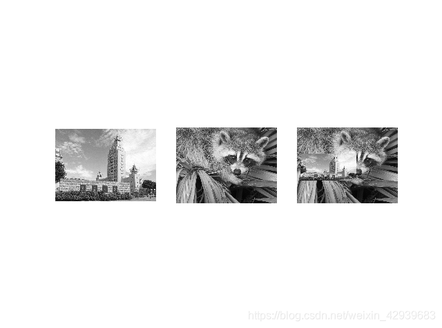
2 图像扭曲

对图像块应用仿射变换，我们将其称为图像扭曲（或者仿射扭曲）。该操作不仅经常在计算机图形学中，而且经常出现在计算机视觉算法总。扭曲的操作可以使用SciPy工具包中的ndimage包来简单完成。

im = array(Image.open('D:\\123\图像处理\Image Processing\Image Processing\\raccoon.jpg').convert('L'))
    H = array([[1.4,0.05,-100],[0.05,1.5,-100],[0,0,1]])
    im2 = ndimage.affine_transform(im, H[:2,:2],(H[0,2],H[1,2]))

    gray()
    subplot(121)
    imshow(im)
    axis('off')
    subplot(122)
    imshow(im2)
    axis('off')
    show()

2.1 图像中的图像

仿射扭曲的一个简单例子是，将图像或者图像的一部分放置在另一幅图像中，是的他们能够和指定的区域或者标记物对齐。

def image_in_image(im1, im2, tp):
    """使用仿射变换将im1放置在im2上，使im1图像的角和tp尽可能的靠近
        tp是齐次表示的，并且是按照从左上角逆时针计算的"""
    
    # 扭曲的点
    m,n = im1.shape[:2]
    fp = array([0,m,m,0],[0,0,n,n],[1,1,1,1])
    
    # 计算仿射变换，并且将其应用于图像im1中
    H = homography.Haffine_from_points(tp, fp)
    im1_t = ndimage.affine_transform(im1,H[:2,:2],
                                     (H[0,2],H[1,2]),im2.shape[:2])
    alpha = (im1_t > 0)
    return (1-alpha)*im2 + alpha*im1_t

im1 = array(Image.open('D:\\123\图像处理\Image Processing\Image Processing\jimei3.jpg').convert('L'))
    im2 = array(Image.open('D:\\123\图像处理\Image Processing\Image Processing\\raccoon.jpg').convert('L'))

    gray()
    subplot(131)
    imshow(im1)
    axis('equal')
    axis('off')
    subplot(132)
    imshow(im2)
    axis('equal')
    axis('off')

    # 选定一些目标点
    tp = array([[264, 538, 540, 264], [40, 36, 605, 605], [1, 1, 1, 1]])

    im3 = image_in_image(im1, im2, tp)
    subplot(133)
    imshow(im3)
    axis('equal')
    axis('off')
    show()

2.2 图像配准

图像配准是对图像进行变换，使变换后的图像能够在常见的坐标系中对齐。配准可以是严格配准，也可以是非严格配准。为了能够进行图像对比和更精细的图像分析，图像配准是一步非常重要的操作。

SIFT算法
SIFT特征匹配算法包括两个阶段:SIFT特征的生成与SIFT特征向量的匹配。
SIFT特征向量的生成算法包括四步：
1.尺度空间极值检测，以初步确定关键点位置和所在尺度。
2.拟和三维二次函数精确确定位置和尺度，同时去除低对比度的关键点和不稳定的边缘响应点。
3.利用关键点领域像素的梯度方向分布特性为每个关键点指定参数方向，使算子具备旋转不变性。
4.生成SIFT特征向量。
SIFT特征向量的匹配
对图像1中的某个关键点，找到其与图像2中欧式距离最近的前两个关键点的距离NN和SCN，如果NN/SCN小于某个比例阈值，则接受这一对匹配点。

基于SIFT的图像配准：

import numpy as np
import cv2

def sift_kp(image):
    gray_image = cv2.cvtColor(image, cv2.COLOR_BGR2GRAY)
    sift = cv2.xfeatures2d_SIFT_create()
    kp, des = sift.detectAndCompute(image, None)
    kp_image = cv2.drawKeypoints(gray_image, kp, None)
    return kp_image, kp, des

def get_good_match(des1, des2):
    bf = cv2.BFMatcher()
    matches = bf.knnMatch(des1, des2, k=2)
    good = []
    for m, n in matches:
        if m.distance < 0.75 * n.distance:
            good.append(m)
    return good

def siftImageAlignment(img1, img2):
    _, kp1, des1 = sift_kp(img1)
    _, kp2, des2 = sift_kp(img2)
    goodMatch = get_good_match(des1, des2)
    if len(goodMatch) > 4:
        ptsA = np.float32([kp1[m.queryIdx].pt for m in goodMatch]).reshape(-1, 1, 2)
        ptsB = np.float32([kp2[m.trainIdx].pt for m in goodMatch]).reshape(-1, 1, 2)
        ransacReprojThreshold = 4
        H, status = cv2.findHomography(ptsA, ptsB, cv2.RANSAC, ransacReprojThreshold);
        # 其中H为求得的单应性矩阵矩阵
        # status则返回一个列表来表征匹配成功的特征点。
        # ptsA,ptsB为关键点
        # cv2.RANSAC, ransacReprojThreshold这两个参数与RANSAC有关
        imgOut = cv2.warpPerspective(img2, H, (img1.shape[1], img1.shape[0]),
                                     flags=cv2.INTER_LINEAR + cv2.WARP_INVERSE_MAP)
    return imgOut, H, status
 
 if __name__=='__main__':

    img1 = cv2.imread('D:\Image\mona_source.png')
    img2 = cv2.imread('D:\Image\mona_target.png')
    while img1.shape[0] > 1000 or img1.shape[1] > 1000:
        img1 = cv2.resize(img1, None, fx=0.5, fy=0.5, interpolation=cv2.INTER_AREA)
    while img2.shape[0] > 1000 or img2.shape[1] > 1000:
        img2 = cv2.resize(img2, None, fx=0.5, fy=0.5, interpolation=cv2.INTER_AREA)

    result, _, _ = siftImageAlignment(img1, img2)
    allImg = np.concatenate((img1, img2, result), axis=1)
    cv2.namedWindow('1', cv2.WINDOW_NORMAL)
    cv2.namedWindow('2', cv2.WINDOW_NORMAL)
    cv2.namedWindow('Result', cv2.WINDOW_NORMAL)
    cv2.imshow('1', img1)
    cv2.imshow('2', img2)
    cv2.imshow('Result', result)
    # cv2.imshow('Result',allImg)
    if cv2.waitKey(200000) & 0xff == ord('q'):
        cv2.destroyAllWindows()
        cv2.waitKey(1)

这里我的OpenCV包是最新版，由于SIFT算法有专利版权OpenCV将sift算法移出了，如果使用旧版本可以运行上面代码。下面是我师姐运行的结果：

3 创建全景图

在同一位置（即图像的照相机位置相同）拍摄的两幅或者多幅图像是单应性相关的。我们经常使用该约束将很多图像缝补起来，拼成一个大的图像来创建全景图像。

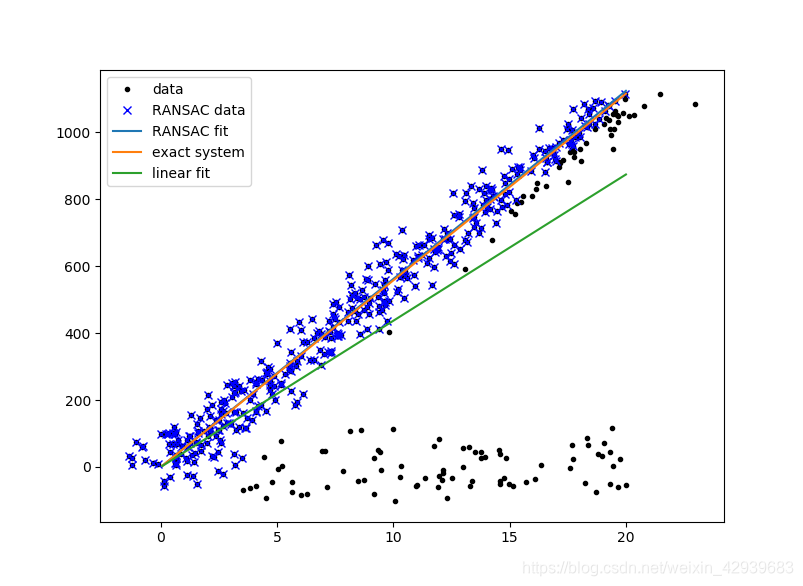
3.1 RANSAC

PANSAC是“RANdom SAmple Consensus”（随机一致性采样）的缩写。该方法是用来找到正确模型来拟合带有噪声数据的迭代方法。给定一个模型，例如点集之间的单应性矩阵，RANSAC基本的思想是，数据中包含着正确的点和噪声点，合理的模型应该能够在描述正确数据点的同时摒弃噪声点。

伪码形式的算法如下所示：
输入：
data —— 一组观测数据
model —— 适应于数据的模型
n —— 适用于模型的最少数据个数
k —— 算法的迭代次数
t —— 用于决定数据是否适应于模型的阀值
d —— 判定模型是否适用于数据集的数据数目
输出：
best_model —— 跟数据最匹配的模型参数（如果没有找到好的模型，返回null）
best_consensus_set —— 估计出模型的数据点
best_error —— 跟数据相关的估计出的模型错误

iterations = 0
best_model = null
best_consensus_set = null
best_error = 无穷大
while ( iterations < k )
maybe_inliers = 从数据集中随机选择n个点
maybe_model = 适合于maybe_inliers的模型参数
consensus_set = maybe_inliers

for ( 每个数据集中不属于maybe_inliers的点 ）
if ( 如果点适合于maybe_model，且错误小于t ）
将点添加到consensus_set
if （ consensus_set中的元素数目大于d ）
已经找到了好的模型，现在测试该模型到底有多好
better_model = 适合于consensus_set中所有点的模型参数
this_error = better_model究竟如何适合这些点的度量
if ( this_error < best_error )
我们发现了比以前好的模型，保存该模型直到更好的模型出现
best_model = better_model
best_consensus_set = consensus_set
best_error = this_error
增加迭代次数
返回 best_model, best_consensus_set, best_error

import numpy
import scipy  # use numpy if scipy unavailable
import scipy.linalg  # use numpy if scipy unavailable

def ransac(data, model, n, k, t, d, debug=False, return_all=False):
    """fit model parameters to data using the RANSAC algorithm

This implementation written from pseudocode found at
http://en.wikipedia.org/w/index.php?title=RANSAC&oldid=116358182

{{{
Given:
    data - a set of observed data points
    model - a model that can be fitted to data points
    n - the minimum number of data values required to fit the model
    k - the maximum number of iterations allowed in the algorithm
    t - a threshold value for determining when a data point fits a model
    d - the number of close data values required to assert that a model fits well to data
Return:
    bestfit - model parameters which best fit the data (or nil if no good model is found)
iterations = 0
bestfit = nil
besterr = something really large
while iterations < k {
    maybeinliers = n randomly selected values from data
    maybemodel = model parameters fitted to maybeinliers
    alsoinliers = empty set
    for every point in data not in maybeinliers {
        if point fits maybemodel with an error smaller than t
             add point to alsoinliers
    }
    if the number of elements in alsoinliers is > d {
        % this implies that we may have found a good model
        % now test how good it is
        bettermodel = model parameters fitted to all points in maybeinliers and alsoinliers
        thiserr = a measure of how well model fits these points
        if thiserr < besterr {
            bestfit = bettermodel
            besterr = thiserr
        }
    }
    increment iterations
}
return bestfit
}}}
"""
    iterations = 0
    bestfit = None
    besterr = numpy.inf
    best_inlier_idxs = None
    while iterations < k:
        maybe_idxs, test_idxs = random_partition(n, data.shape[0])
        maybeinliers = data[maybe_idxs, :]
        test_points = data[test_idxs]
        maybemodel = model.fit(maybeinliers)
        test_err = model.get_error(test_points, maybemodel)
        also_idxs = test_idxs[test_err < t]  # select indices of rows with accepted points
        alsoinliers = data[also_idxs, :]
        if debug:
            print 'test_err.min()', test_err.min()
            print 'test_err.max()', test_err.max()
            print 'numpy.mean(test_err)', numpy.mean(test_err)
            print 'iteration %d:len(alsoinliers) = %d' % (
                iterations, len(alsoinliers))
        if len(alsoinliers) > d:
            betterdata = numpy.concatenate((maybeinliers, alsoinliers))
            bettermodel = model.fit(betterdata)
            better_errs = model.get_error(betterdata, bettermodel)
            thiserr = numpy.mean(better_errs)
            if thiserr < besterr:
                bestfit = bettermodel
                besterr = thiserr
                best_inlier_idxs = numpy.concatenate((maybe_idxs, also_idxs))
        iterations += 1
    if bestfit is None:
        raise ValueError("did not meet fit acceptance criteria")
    if return_all:
        return bestfit, {'inliers': best_inlier_idxs}
    else:
        return bestfit


def random_partition(n, n_data):
    """return n random rows of data (and also the other len(data)-n rows)"""
    all_idxs = numpy.arange(n_data)
    numpy.random.shuffle(all_idxs)
    idxs1 = all_idxs[:n]
    idxs2 = all_idxs[n:]
    return idxs1, idxs2


class LinearLeastSquaresModel:
    """linear system solved using linear least squares

    This class serves as an example that fulfills the model interface
    needed by the ransac() function.

    """

    def __init__(self, input_columns, output_columns, debug=False):
        self.input_columns = input_columns
        self.output_columns = output_columns
        self.debug = debug

    def fit(self, data):
        A = numpy.vstack([data[:, i] for i in self.input_columns]).T
        B = numpy.vstack([data[:, i] for i in self.output_columns]).T
        x, resids, rank, s = numpy.linalg.lstsq(A, B)
        return x

    def get_error(self, data, model):
        A = numpy.vstack([data[:, i] for i in self.input_columns]).T
        B = numpy.vstack([data[:, i] for i in self.output_columns]).T
        B_fit = scipy.dot(A, model)
        err_per_point = numpy.sum((B - B_fit) ** 2, axis=1)  # sum squared error per row
        return err_per_point


def test():
    # generate perfect input data

    n_samples = 500
    n_inputs = 1
    n_outputs = 1
    A_exact = 20 * numpy.random.random((n_samples, n_inputs))
    perfect_fit = 60 * numpy.random.normal(size=(n_inputs, n_outputs))  # the model
    B_exact = scipy.dot(A_exact, perfect_fit)
    assert B_exact.shape == (n_samples, n_outputs)

    # add a little gaussian noise (linear least squares alone should handle this well)
    A_noisy = A_exact + numpy.random.normal(size=A_exact.shape)
    B_noisy = B_exact + numpy.random.normal(size=B_exact.shape)

    if 1:
        # add some outliers
        n_outliers = 100
        all_idxs = numpy.arange(A_noisy.shape[0])
        numpy.random.shuffle(all_idxs)
        outlier_idxs = all_idxs[:n_outliers]
        non_outlier_idxs = all_idxs[n_outliers:]
        A_noisy[outlier_idxs] = 20 * numpy.random.random((n_outliers, n_inputs))
        B_noisy[outlier_idxs] = 50 * numpy.random.normal(size=(n_outliers, n_outputs))

    # setup model

    all_data = numpy.hstack((A_noisy, B_noisy))
    input_columns = range(n_inputs)  # the first columns of the array
    output_columns = [n_inputs + i for i in range(n_outputs)]  # the last columns of the array
    debug = True
    model = LinearLeastSquaresModel(input_columns, output_columns, debug=debug)

    linear_fit, resids, rank, s = numpy.linalg.lstsq(all_data[:, input_columns], all_data[:, output_columns])

    # run RANSAC algorithm
    ransac_fit, ransac_data = ransac(all_data, model,
                                     5, 5000, 7e4, 50,  # misc. parameters
                                     debug=debug, return_all=True)
    if 1:
        import pylab

        sort_idxs = numpy.argsort(A_exact[:, 0])
        A_col0_sorted = A_exact[sort_idxs]  # maintain as rank-2 array

        if 1:
            pylab.plot(A_noisy[:, 0], B_noisy[:, 0], 'k.', label='data')
            pylab.plot(A_noisy[ransac_data['inliers'], 0], B_noisy[ransac_data['inliers'], 0], 'bx',
                       label='RANSAC data')
        else:
            pylab.plot(A_noisy[non_outlier_idxs, 0], B_noisy[non_outlier_idxs, 0], 'k.', label='noisy data')
            pylab.plot(A_noisy[outlier_idxs, 0], B_noisy[outlier_idxs, 0], 'r.', label='outlier data')
        pylab.plot(A_col0_sorted[:, 0],
                   numpy.dot(A_col0_sorted, ransac_fit)[:, 0],
                   label='RANSAC fit')
        pylab.plot(A_col0_sorted[:, 0],
                   numpy.dot(A_col0_sorted, perfect_fit)[:, 0],
                   label='exact system')
        pylab.plot(A_col0_sorted[:, 0],
                   nu  mpy.dot(A_col0_sorted, linear_fit)[:, 0],
                   label='linear fit')
        pylab.legend()
        pylab.show()
if __name__ == '__main__':
    test()

RANSAC算法的可能变化包括以下几种：
（1）如果发现了一种足够好的模型（该模型有足够小的错误率），则跳出主循环。这样可能会节约计算额外参数的时间。
（2）直接从maybe_model计算this_error，而不从consensus_set重新估计模型。这样可能会节约比较两种模型错误的时间，但可能会对噪声更敏感。

其实核心就是随机性和假设性。随机性用于减少计算了，那个循环次数就是利用正确数据出现的概率。所谓的假设性，就是说随机抽出来的数据我都认为是正确的，并以此去计算其他点，获得其他满足变换关系的点，然后利用投票机制，选出获票最多的那一个变换。

RANSAC的优点是它能鲁棒的估计模型参数。例如，它能从包含大量局外点的数据集中估计出高精度的参数。RANSAC的缺点是它计算参数的迭代次数没有上限；如果设置迭代次数的上限，得到的结果可能不是最优的结果，甚至可能得到错误的结果。RANSAC只有一定的概率得到可信的模型，概率与迭代次数成正比。RANSAC的另一个缺点是它要求设置跟问题相关的阀值。
RANSAC只能从特定的数据集中估计出一个模型，如果存在两个（或多个）模型，RANSAC不能找到别的模型。

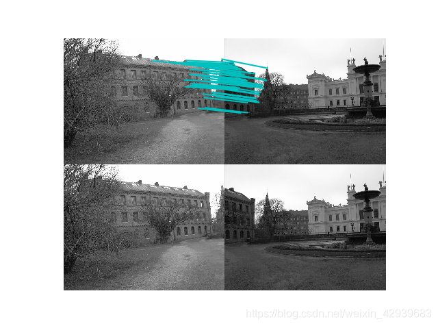
3.2 稳健的单应性矩阵估计

我们在任何模型中都可以使用 RANSAC 模块。在使用 RANSAC 模块时，我们只需要在相应 Python 类中实现 fit() 和 get_error() 方法，剩下就是正确地使用 ransac.py，我们这里使用可能的对应点集来自动找到用于全景图像的单应性矩阵。下面是使用SIFT特征自动找到匹配对应。

featname = ['Univ'+str(i+1)+'.sift' for i in range(5)]
    imname = ['Univ'+str(i+1)+'.jpg' for i in range(5)]
    im = [array(Image.open(imname[i]).convert('L')) for i in range(5)]
    l = {}
    d = {}
    for i in range(5):
        # process_image(imname[i], featname[i])
        l[i],d[i] = read_features_from_file(featname[i])

    matches = {}
    for i in range(4):
        matches[i] = match(d[i+1], d[i])

    figure()
    gray()
    for i in range(4):
        plot_matches(im[i+1], im[i], l[i+1], l[i], matches[i], show_below=True)
        figure()
    show()

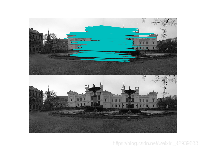
3.3 拼接图像

估计出图像间的单应性矩阵（使用RANSAC算法），现在我们需要将所有的图像扭曲到一个公共的图像平面上。通常，这里的公共平面为中心图像平面（否则需要大量变形）。一种方法是创建一个很大的图像，比如图像中全部填充0，使其和中心图像平行，然后将所有的图像扭曲到上面。由于我们所有的图像是由照相机水平旋转拍摄的，因此我们可以使用一个较简单的步骤：将中心图像左边或者右边的区域填充为0，以便为扭曲的图像腾出空间。

from pylab import *
from numpy import *
from PIL import Image

# If you have PCV installed, these imports should work
from PCV.geometry import homography, warp
from PCV.localdescriptors import sift

# 将匹配转换成齐次坐标点的函数
def convert_points(j):
    ndx = matches[j].nonzero()[0]
    fp = homography.make_homog(l[j + 1][ndx, :2].T)
    ndx2 = [int(matches[j][i]) for i in ndx]
    tp = homography.make_homog(l[j][ndx2, :2].T)

    # switch x and y - TODO this should move elsewhere
    fp = vstack([fp[1], fp[0], fp[2]])
    tp = vstack([tp[1], tp[0], tp[2]])
    return fp, tp

if __name__=='__main__':

    featname = ['Univ' + str(i + 1) + '.sift' for i in range(5)]
    imname = ['Univ' + str(i + 1) + '.jpg' for i in range(5)]
    im = [array(Image.open(imname[i]).convert('L')) for i in range(5)]
    l = {}
    d = {}
    for i in range(5):
        # process_image(imname[i], featname[i])
        l[i], d[i] = sift.read_features_from_file(featname[i])

    matches = {}
    for i in range(4):
        matches[i] = sift.match(d[i + 1], d[i])

    # figure()
    # gray()
    # for i in range(4):
    #     sift.plot_matches(im[i + 1], im[i], l[i + 1], l[i], matches[i], show_below=True)
    #     figure()
    # show()

    # 估计单应性矩阵
    model = homography.RansacModel()

    fp, tp = convert_points(1)
    H_12 = homography.H_from_ransac(fp, tp, model)[0]  # im 1 to 2

    fp, tp = convert_points(0)
    H_01 = homography.H_from_ransac(fp, tp, model)[0]  # im 0 to 1

    tp, fp = convert_points(2)  # NB: reverse order
    H_32 = homography.H_from_ransac(fp, tp, model)[0]  # im 3 to 2

    tp, fp = convert_points(3)  # NB: reverse order
    H_43 = homography.H_from_ransac(fp, tp, model)[0]  # im 4 to 3

    # 扭曲图像
    delta = 2000  # for padding and translation用于填充和平移

    im1 = array(Image.open(imname[1]), "uint8")
    im2 = array(Image.open(imname[2]), "uint8")
    im_12 = warp.panorama(H_12,im1,im2,delta,delta)

    im1 = array(Image.open(imname[0]), "f")
    im_02 = warp.panorama(dot(H_12,H_01),im1,im_12,delta,delta)

    im1 = array(Image.open(imname[3]), "f")
    im_32 = warp.panorama(H_32,im1,im_02,delta,delta)

    im1 = array(Image.open(imname[4]), "f")
    im_42 = warp.panorama(dot(H_32,H_43),im1,im_32,delta,2*delta)

    figure()
    imshow(array(im_42, "uint8"))
    axis('off')
    show()

这里我没有使用书上给的源码，使用了PVC，其中由于PVC的包中很多是跟Python2所兼容的可以会出一些错误，比如print变为print()。这里如果遇到提示如 ModuleNotFoundError: No module named ‘matplotlib.delaunay’。解决方法如下：https://blog.csdn.net/weixin_42648848/article/details/88667243