使用Pytorch和Matplotlib可视化卷积神经网络的特征

在处理图像和图像数据时，CNN是最常用的架构。卷积神经网络已经被证明在深度学习和计算机视觉领域提供了许多最先进的解决方案。没有CNN，图像识别、目标检测、自动驾驶汽车就不可能实现。

但当归结到CNN如何看待和识别他们所做的图像时，事情就变得更加棘手了。

• CNN如何判断一张图片是猫还是狗?
• 在图像分类问题上，是什么让CNN比其他模型更强大?
• 他们在图像中看到了什么?

这是我第一次了解CNN时的一些问题。问题会随着你的深入而增加。

那时候我听说过过滤器和特性映射，但不知道它们是什么，它们的作用是什么。后来我知道他们是什么，但不知道他们长什么样子，但现在我知道了。在处理深度卷积网络时，过滤器和特征映射很重要。滤镜是使特征被复制的东西，也是模型看到的东西。

什么是CNN的滤镜和特性映射?

过滤器是使用反向传播算法学习的一组权值。如果你做了很多实际的深度学习编码，你可能知道它们也被称作核。过滤器的尺寸可以是3×3，也可以是5×5，甚至7×7。

过滤器在一个CNN层学习检测抽象概念，如人脸的边界，建筑物的边缘等。通过叠加越来越多的CNN层，我们可以从一个CNN中得到更加抽象和深入的信息。

特性映射是我们通过图像的像素值进行滤波后得到的结果。这就是模型在图像中看到的这个过程叫做卷积运算。将feature map可视化的原因是为了加深对CNN的了解。

选择模型

我们将使用ResNet-50神经网络模型来可视化过滤器和特征图。使用ResNet-50模型来可视化过滤器和特征图并不理想。原因是resnet模型总的来说有点复杂。遍历内部卷积层会变得非常困难。但是在本篇文章中您将了解如何访问复杂体系结构的内部卷积层后，您将更加适应使用类似的或更复杂的体系结构。

我使用的图片来自pexels。这是我为了训练我的人脸识别分类器而收集的一幅图像。

模型结构

乍一看，模型的结构可能令人生畏，但要得到我们想要的东西确实很容易。通过了解如何提取这个模型的层，您将能够提取更复杂模型的层。下面是模型结构。

ResNet(
  (conv1): Conv2d(3, 64, kernel_size=(7, 7), stride=(2, 2), padding=(3, 3), bias=False)
  (bn1): BatchNorm2d(64, eps=1e-05, momentum=0.1, affine=True, track_running_stats=True)
  (relu): ReLU(inplace=True)
  (maxpool): MaxPool2d(kernel_size=3, stride=2, padding=1, dilation=1, ceil_mode=False)
  (layer1): Sequential(
    (0): Bottleneck(
      (conv1): Conv2d(64, 64, kernel_size=(1, 1), stride=(1, 1), bias=False)
      (bn1): BatchNorm2d(64, eps=1e-05, momentum=0.1, affine=True, track_running_stats=True)
      (conv2): Conv2d(64, 64, kernel_size=(3, 3), stride=(1, 1), padding=(1, 1), bias=False)
      (bn2): BatchNorm2d(64, eps=1e-05, momentum=0.1, affine=True, track_running_stats=True)
      (conv3): Conv2d(64, 256, kernel_size=(1, 1), stride=(1, 1), bias=False)
      (bn3): BatchNorm2d(256, eps=1e-05, momentum=0.1, affine=True, track_running_stats=True)
      (relu): ReLU(inplace=True)
      (downsample): Sequential(
        (0): Conv2d(64, 256, kernel_size=(1, 1), stride=(1, 1), bias=False)
        (1): BatchNorm2d(256, eps=1e-05, momentum=0.1, affine=True, track_running_stats=True)
      )
    )
    (1): Bottleneck(
      (conv1): Conv2d(256, 64, kernel_size=(1, 1), stride=(1, 1), bias=False)
      (bn1): BatchNorm2d(64, eps=1e-05, momentum=0.1, affine=True, track_running_stats=True)
      (conv2): Conv2d(64, 64, kernel_size=(3, 3), stride=(1, 1), padding=(1, 1), bias=False)
      (bn2): BatchNorm2d(64, eps=1e-05, momentum=0.1, affine=True, track_running_stats=True)
      (conv3): Conv2d(64, 256, kernel_size=(1, 1), stride=(1, 1), bias=False)
      (bn3): BatchNorm2d(256, eps=1e-05, momentum=0.1, affine=True, track_running_stats=True)
      (relu): ReLU(inplace=True)
...
(2): Bottleneck(
      (conv1): Conv2d(2048, 512, kernel_size=(1, 1), stride=(1, 1), bias=False)
      (bn1): BatchNorm2d(512, eps=1e-05, momentum=0.1, affine=True, track_running_stats=True)
      (conv2): Conv2d(512, 512, kernel_size=(3, 3), stride=(1, 1), padding=(1, 1), bias=False)
      (bn2): BatchNorm2d(512, eps=1e-05, momentum=0.1, affine=True, track_running_stats=True)
      (conv3): Conv2d(512, 2048, kernel_size=(1, 1), stride=(1, 1), bias=False)
      (bn3): BatchNorm2d(2048, eps=1e-05, momentum=0.1, affine=True, track_running_stats=True)
      (relu): ReLU(inplace=True)
    )
  )
  (avgpool): AdaptiveAvgPool2d(output_size=(1, 1))
  (fc): Linear(in_features=2048, out_features=1000, bias=True)

提取CNN层

conv_layers = []
model_weights = []
model_children = list(models.resnet50().children())
counter = 0

for i in range(len(model_children)):
    if type(model_children[i]) == nn.Conv2d:
        counter += 1
        model_weights.append(model_children[i].weight)
        conv_layers.append(model_children[i])
    elif type(model_children[i]) == nn.Sequential:
        for j in range(len(model_children[i])):
            for child in model_children[i][j].children():
                if type(child) == nn.Conv2d:
                    counter += 1
                    model_weights.append(child.weight)
                    conv_layers.append(child)

1. 首先，在第4行，我们初始化一个计数器变量，以跟踪卷积层的数量。
2. 从第6行开始，我们将遍历ResNet-50模型的所有层。
3. 具体来说，我们在三层嵌套中检查卷积层
4. 第7行，检查模型的直接子层中是否有卷积层。
5. 然后从第10行开始，我们检查序列块中的瓶颈层是否包含任何卷积层。
6. 如果上述两个条件中有一个满足，那么我们将该子节点和权值分别附加到conv_layers和model_weights，

上面的代码很简单并且不言自明，但是它仅限于已经存在的模型，比如其他resnet模型resnet-18、34、101、152。对于自定义模型，情况将有所不同，假设在另一个连续层中有一个连续层，如果有一个CNN层，程序将不检查它。这就是我编写的extract .py模块可能有用的地方。

Extractor类

Extractor类可以找到每一个CNN层(除了下采样层)，包括它们在任何resnet模型以及几乎在任何自定义resnet和vgg模型中的权重。它不局限于CNN层，它可以找到线性层，如果提到了下采样层的名字，它也可以找到。它还可以提供一些有用的信息，如CNN的数量、模型中的线性层和顺序层。

如何使用

在Extractor类中，模型参数接受模型，而DS_layer_name参数是可选的。DS_layer_name参数用于查找下采样层，通常在resnet层中名称为“downsample”，因此它保持为默认值。

extractor = Extractor(model = resnet, DS_layer_name = 'downsample') 

extractor.activate()）是激活程序。
extractor.info()可以查看里面的方法

{'Down-sample layers name': 'downsample', 'Total CNN Layers': 49, 'Total Sequential Layers': 4, 'Total Downsampling Layers': 4, 'Total Linear Layers': 1, 'Total number of Bottleneck and Basicblock': 16, 'Total Execution time': '0.00137 sec'}

访问权重和层

extractor.CNN_layers -----> Gives all the CNN layers in a model
extractor.Linear_layers --> Gives all the Linear layers in a model
extractor.DS_layers ------> Gives all the Down-sample layers in a model if there are any
extractor.CNN_weights ----> Gives all the CNN layer's weights in a model
extractor.Linear_weights -> Gives all the Linear layer's weights in a model

没有任何编码，你可以得到CNN和线性层和他们的权值在几乎每个resnet模型。下面是类的方法

def activate(self):
        """Activates the algorithm"""

        start = time.time()
        self.__Layer_Extractor(self.model_children)
        self.__Verbose()
        self.__ex_time = str(round(time.time() - start, 5)) + ' sec'
def __Append(self, layer, Linear=False):
        """
        This function will append the layers weights and
        the layer itself to the appropriate variables
        params: layer: takes in CNN or Linear layer
        returns: None
        """

        if Linear:
            self.Linear_weights.append(layer.weight)
            self.Linear_layers.append(layer)

        else:
            self.CNN_weights.append(layer.weight)
            self.CNN_layers.append(layer)
def __Layer_Extractor(self, layers):
        """
        This function(algorithm) finds CNN and linear layer in a Sequential layer
        params: layers: takes in either CNN or Sequential or linear layer
        return: None
        """

        for x in range(len(layers)):

            if type(layers[x]) == nn.Sequential:
                # Calling the fn to loop through the layer to get CNN layer
                self.__Layer_Extractor(layers[x])
                self.__no_sq_layers += 1

            if type(layers[x]) == nn.Conv2d:
                self.__Append(layers[x])

            if type(layers[x]) == nn.Linear:
                self.__Append(layers[x], True)

            # This statement makes sure to get the down-sampling layer in the model
            if self.DS_layer_name in layers[x]._modules.keys():
                self.DS_layers.append(layers[x]._modules[self.DS_layer_name])

            # The below statement will loop throgh the containers and append it
            if isinstance(layers[x], (self.__bottleneck, self.__basicblock)):
                self.__no_containers += 1
                for child in layers[x].children():
                    if type(child) == nn.Conv2d:
                        self.__Append(child)

可视化

卷积层

在这里，我们将可视化卷积层过滤器。为了简单起见，我们将只可视化第一个卷积层的过滤器。

# Visualising the filters
plt.figure(figsize=(35, 35))
for index, filter in enumerate(extractor.CNN_weights[0]):
    plt.subplot(8, 8, index + 1)
    plt.imshow(filter[0, :, :].detach(), cmap='gray')
    plt.axis('off')

plt.show()

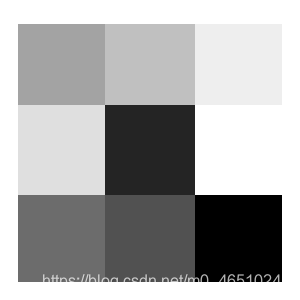
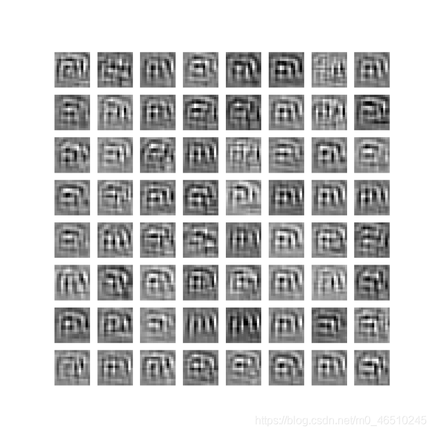
第一层的滤波器尺寸为7×7，有64个通道(隐藏层)。

来自训练好的resnet-50模型的7×7个过滤器

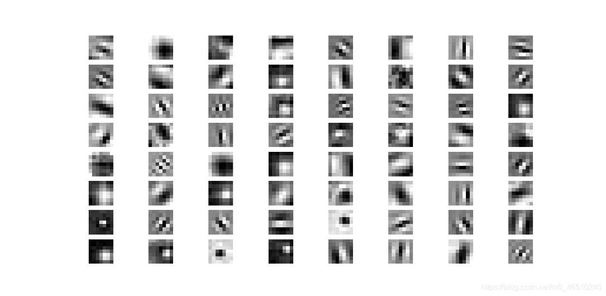
每个小方框的像素值在0到255之间。0是完全黑的255是白色的。范围可以是不同的，比如0到1或-1到1，以0为平均值。

特征映射

为了使特征映射形象化，首先需要将图像转换为张量图像。利用torchvision的变换，可以将图像归一化并转换为张量。

# Filter Map
img = cv.cvtColor(cv.imread('filtermap/5.png'), cv.COLOR_BGR2RGB)
#transforms is imported as t
img = t.Compose([
    t.ToPILImage(),
    t.Resize((128, 128)),
    # t.Grayscale(),
    t.ToTensor(),
    t.Normalize(0.5, 0.5)])(img).unsqueeze(0)
#LAST LINE
t.Normalize(0.5, 0.5)])(img).unsqueeze(0)

变换后的最后一行表示将变换应用于图像。您可以创建一个新变量，然后应用它，但是一定要更改变量名。unsqueze（0）是给张量img增加一个额外的维数。添加批处理维度是一个重要步骤。现在图像的大小不是[3，128，128]，而是[1，3，128，128]，这表示批处理中只有一个图像。

将图像输入每个卷积层

下面的代码将图像通过每个卷积层。

featuremaps = [extractor.CNN_layers [0] (img)]
len(extractor.CNN_layers):
featuremaps.append (extractor.CNN_layers [x] (featuremaps [1]))

我们将首先把图像作为输入,传递给第一个卷积层。在此之后，我们将使用for循环将最后一层的输出传递给下一层，直到到达最后一个卷积层。

• 在第1行，我们将图像作为第一个卷积层的输入。
• 然后我们使用for循环从第二层循环到最后一层卷积。
• 我们将最后一层的输出作为下一个卷积层的输入(featuremaps[-1])。
• 另外，我们将每个层的输出附加到featuremaps列表中。

特征的可视化

这是最后一步。我们将编写代码来可视化特征映射。注意，最后的cnn层有很多feature map，范围在512到2048之间。但是我们将只从每一层可视化64个特征图，否则将使输出真正地混乱。

# Visualising the featuremaps
for x in range(len(featuremaps)):
    plt.figure(figsize=(30, 30))
    layers = featuremaps[x][0, :, :, :].detach()
    for i, filter in enumerate(layers):
        if i == 64:
            break
        plt.subplot(8, 8, i + 1)
        plt.imshow(filter, cmap='gray')
        plt.axis('off')

    # plt.savefig('featuremap%s.png'%(x))

plt.show()

• 从第2行开始，我们遍历feature remaps。
• 然后我们得到的层是featuremaps[x][0，:，:，:].detach()。
• 从第5行开始，我们遍历每个层中的过滤器。如果它是第64个特征图，我们就跳出了循环。
• 在此之后，我们绘制feature map，并在必要时保存它们。

结果

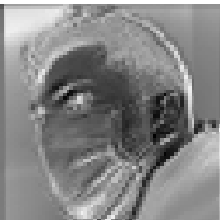
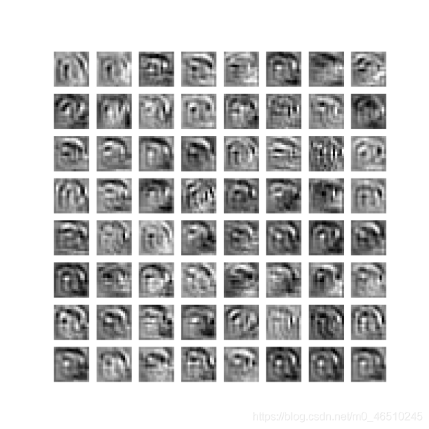
可以看到，在创建图像的feature map时，不同的滤镜聚焦于不同的方面。

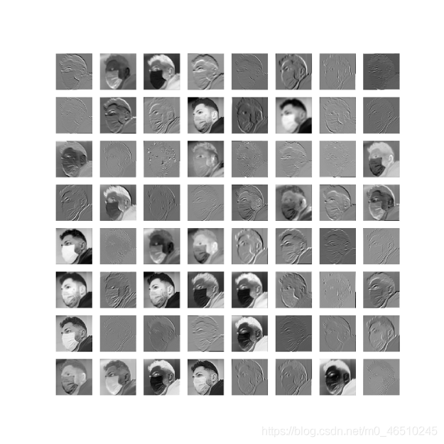
一些特征地图聚焦于图像的背景。另一些人则创建了图像的轮廓。一些滤镜创建的特征地图，背景是黑暗的，但图像的脸是明亮的。这是由于过滤器的相应权重。从上面的图像可以很清楚地看出，在深层，神经网络可以看到输入图像非常详细的特征图。

让我们看看其他一些特征。

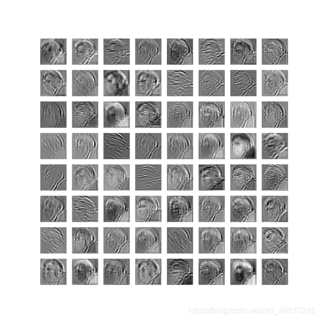
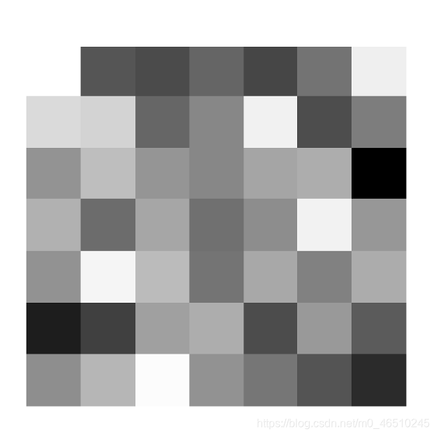
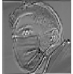
ResNet-50模型的第20和第10卷积层的Feature map

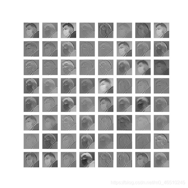
ResNet-50模型第40和第30卷积层的Feature map

你可以观察到，当图像通过层的进展，细节从图像慢慢消失。它们看起来像噪音，但在这些特征地图中肯定有一种模式是人眼无法察觉的，但神经网络可以。

当图像到达最后的卷积层时，人类就不可能知道那是什么了。最后一层输出对于最后的全连接的神经元非常重要，这些神经元基本上构成了卷积神经网络的分类层。

代码：https://github.com/Rahul0128/Visualizing-Filters-and-Feature-Maps-in-Convolutional-Neural-Networks-using-PyTorch

作者 Rahulpillai

deephub翻译组