自然语言处理基本概念、词向量发展、语言模型

1. 基本概念

1. 1 语料库&词典

• 一般语料库就是很多篇文章（可能一篇文章有好几句话，也可能只有一句话），在实际业务中，每篇文章一般要先进行分词
• 词典：语料库中词的种类数，即有多少个词，一般用|V|表示
• 树中根节点就是最上面那个，叶子结点就是结果（如分类的标签），结点泛指所有（包括根节点、叶子结点）

2. 词向量：one-hot & 特征、标签的ont-hot编码

2.1 词向量one-hot

对于训练数据，如
[[the, cat, is, running],
[the, dog, is, cute, that, dog, is, smart]]
one_hot就是词出现一次就打上标签1。上述训练数据转换之后为

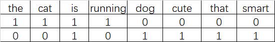
可以看到最上面一行就是词的种类，第二行是第一个样本的one-hot转换，第三行是第二个样本的ont-hot转换。只要出现了该词，就打1，无论出现了多少次。
ont-hot首先没考虑词的顺序，也没考虑词出现的次数。且容易造成很大的稀疏矩阵。

• one-hot代码实现

from sklearn.feature_extraction.text import CountVectorizer
corpus = [
     'This is the first document.',   # 输入的文本是一个字符串
     'This document is the second document.',
     'And this is the third one.',
     'Is this the first document?']
vectorizer = CountVectorizer(binary=True)    # 注这里binary一定为True，否则就不是one-hot了
X = vectorizer.fit_transform(corpus)
print(vectorizer.get_feature_names())
print(X.toarray())

['and', 'document', 'first', 'is', 'one', 'second', 'the', 'third', 'this']
[[0 1 1 1 0 0 1 0 1]
 [0 1 0 1 0 1 1 0 1]
 [1 0 0 1 1 0 1 1 1]
 [0 1 1 1 0 0 1 0 1]]        

2.2 特征、标签的ont-hot编码

• 除了上述将整个文本用one-hot表示，机器学习中还会遇到将类别特征进行ont-hot编码。如多元线性回归中，其中一个特征是性别（男，女），这时，我们就想让男、女各单独作为一个特征，如果是男，男的特征就为1，相应的女的特征就为0。具体实现如下

# sklearn 实现---1
# sklearn中OneHotEncoder可以同时对多列特征就行one-hot处理
from sklearn.preprocessing import OneHotEncoder
enc = OneHotEncoder(handle_unknown='ignore')
X = [['Male', 'a', 'c'], 
     ['Female', 'b', 'd'], 
     ['Female', 'c', 'e']]
enc.fit(X)  # 第一列是性别特征，可以分成两列，分别代表是不是男，是不是女；其他两列亦同。
print(enc.categories_)
enc.transform([['Female', 1, 2],    
               ['Male', 'e', 'e']]).toarray()  # 当transform出现训练集没有的，如本来是男女，突然出现一个“unknown”，这时男、女两列都为0，因为handle_unknown='ignore'，还可以设置成’error’
               # 即出现训练集没有的就报错

[array(['Female', 'Male'], dtype=object), array(['a', 'b', 'c'], dtype=object), array(['c', 'd', 'e'], dtype=object)]
array([[1., 0., 0., 0., 0., 0., 0., 0.],
       [0., 1., 0., 0., 0., 0., 0., 1.]])

# pandas实现
s = pd.Series(['male', 'female', 'male', 'female', np.nan]) 
pd.get_dummies(s)

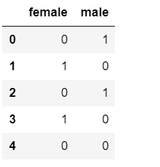
上面pandas实现的时候是以特征性别为例的，如果换成标签，就是对标签进行one-hot编码

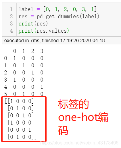
标签的one-hot编码，pytorch、tensorflow（包括keras）都实现了自己的api，在此不再赘述。

3. 词向量：词袋

上一章one-hot词向量不考虑单词出现的次数，如

[[the, cat, is, running],
[the, dog, is, cute, that, dog, is, smart]]
虽然第二句话，the出现了两次，但最终the仍表示成1。
词袋就是在one-hot基础上发展而来的，只是不再仅仅表示成1，而是单词出现的个数。此时该例的结果为

• 代码实现

from sklearn.feature_extraction.text import CountVectorizer
corpus = [
     'the cat is running',
     'this dog is cute that dog is smart']
vectorizer = CountVectorizer(binary=False)   # binary改为False就是统计出现的次数，即词袋了 
X = vectorizer.fit_transform(corpus)
print(vectorizer.get_feature_names())
print(X.toarray())

['cat', 'cute', 'dog', 'is', 'running', 'smart', 'that', 'the', 'this']
[[1 0 0 1 1 0 0 1 0]
 [0 1 2 2 0 1 1 0 1]]

4. 词向量：n-gram & 语言模型：n-gram

4.1 词向量

还是该例
[[the, cat, is, running],
[this, dog, is, cute, that, dog, is, smart]]
上两章都是以一个单词为单元统计是否出现或出现的次数，但有时两个单词可能更有意义，如do not，统计do not出现的次数更加符合实际，这就是n-gram词向量表示。下面从代码中具体理解，依然用的是sklearn的CountVectorizer这个API

from sklearn.feature_extraction.text import CountVectorizer
corpus = ['the cat is running',
         'this dog is cute, that dog is smart']
vectorizer = CountVectorizer(ngram_range=(1,2)) # (1,2)表示统计单个词出现的次数及两个词一起出现的次数  
X = vectorizer.fit_transform(corpus)
print(vectorizer.get_feature_names())
print(X.toarray())

['cat', 'cat is', 'cute', 'cute that', 'dog', 'dog is', 'is', 'is cute', 'is running', 'is smart', 'running', 'smart', 'that', 'that dog', 'the', 'the cat', 'this', 'this dog']
[[1 1 0 0 0 0 1 0 1 0 1 0 0 0 1 1 0 0]
 [0 0 1 1 2 2 2 1 0 1 0 1 1 1 0 0 1 1]]

4.2 sklearn.feature_extraction.text.CountVectorizer讲解

one-hot向量、词袋向量、n-gram向量都是用的该API，下面就对该API详细介绍一下

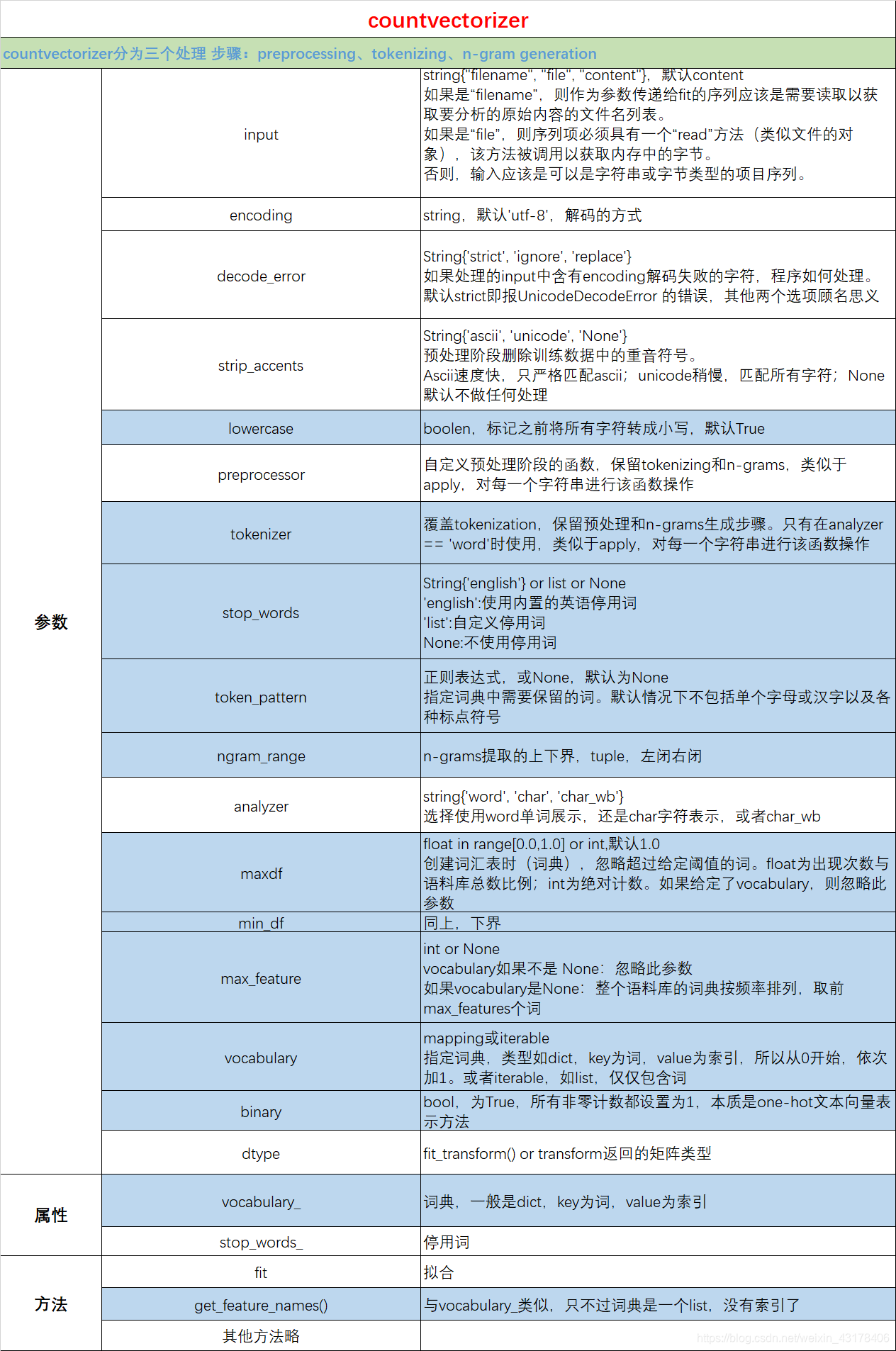
蓝色填充表示比较重要。其中，重音可参考https://zimt8.com/questions/517923/

from sklearn.feature_extraction.text import CountVectorizer
corpus = [
     'a fine cut',
     '他 喜欢 动物']
vectorizer = CountVectorizer(binary=False, analyzer='word', ) 
X = vectorizer.fit_transform(corpus)
print(vectorizer.get_feature_names())
print(X.toarray())

['cut', 'fine', '动物', '喜欢']
[[1 1 0 0]
 [0 0 1 1]]

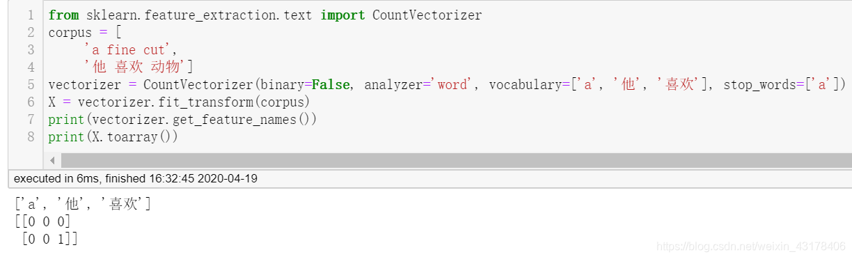
从结果我们可以看到，在生成的词典里没有a、他。原因如下：
没有指定vocabulary，即生成的词典需要CountVectorizer根据分词结果及max_df、max_features等自己生成；此外没有指定tokenizer，及分词函数没有指定；在上述两个参数都没指定的情况下，就会看参数token_pattern，而我们又没有指定，那么CountVectorizer就会以单个字母或汉字及各种标点符号当做分词的标准。所以上述代码没有a和他。如果想让a和他也加入到生成的词典中，有三种方法

• 指定vocabulary，此时tokenizer/token_pattern/stop_words/max_df等都无效，即和分词有关的参数都无效。可以看到最终生成的词典只有我们参数中指定的a/他/喜欢
  
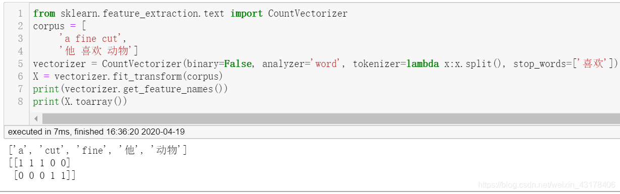
• 在不指定vocabulary的情况下，指定tokenizer，即指定分词的函数，此时stop_words等还是有效的，因为我们指定这个参数，仅仅是确定如何分词，不影响最终生成的词典还需要去停用词，去不满足max_features等的词，但是token_pattern无效
  
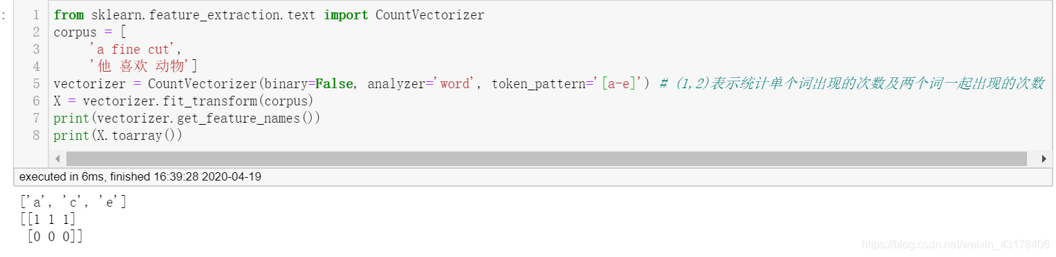
• 在不指定vocabulary和tokenizer的情况下，指定token_pattern，该参数和tokenizer相似，指定了要保留哪些词，需要用正则表达式。
  

4.3 语言模型：n-gram

在讲n-gram之前，首先了解什么是朴素贝叶斯，而朴素贝叶斯模型和n-gram模型都属于语言模型的一种

4.3.1 语言模型

语言模型就是计算一个句子的概率模型。比如以下两句话
今天天气很好，我们出去玩吧。
今天天气很好，俺们出去玩吧。
如果第一句话出现的概率为80%，第二句话出现的概率为60%，那么我们认为第一句话更为合理。
如何计算一句话出现的概率？
假如计算"我爱你"这句话出现的概率
令s=“我爱你”
那么
$p(s)=p(我)p(爱|我)p(你|我爱)$
一般得，一句话$s=({\omega }_1,{\omega }_2,...,{\omega }_n)$出现的概率为：
$$p(s)=p({\omega }_1)p({\omega }_2|{\omega }_1)p({\omega }_3|{\omega }_1,{\omega }_2)...p({\omega }_n|{\omega }_1,{\omega }_2,...,{\omega }_{n-1})$$
语言模型的缺点：

• 参数空间过大，条件概率$p({\omega }_n|{\omega }_1,{\omega }_2,...,{\omega }_{n-1})$d的可能性太多，无法估算
• 数据稀疏严重，对于非常多词的组合，在语料库中都没有出现，依据最大似然估计得到的概率将为0

4.3.2 n-gram

上一小节提到参数空间过大的问题，因此引入一个假设：任意一个词出现的概率只与它前面出现的有限的一个或几个词有关。
假设一个词出现的概率只有他前面的一个词有关，这种假设被称为马尔科夫假设。此时S的概率变为
$$p({\omega }_1,...{\omega }_n)=p({\omega }_1)p({\omega }_2|{\omega }_1)p({\omega }_3|{\omega }_2)...p({\omega }_n|{\omega }_{n-1})$$
接下来的问题变成估计条件概率$p({\omega }_i|{\omega }_{i-1})$:
$$p({\omega }_i|{\omega }_{i-1})=\frac{p({\omega }_i,{\omega }_{i-1})}{p({\omega }_{i-1})}$$
当样本量很大时，基于大数定律，一个短语或者词语出现的概率可以用其频率来表示，即：
$$p({\omega }_i|{\omega }_{i-1})=\frac{count({\omega }_i,{\omega }_{i-1})}{count({\omega }_{i-1})}$$
举个例子，假设语料库词语出现的次数如下表所示：

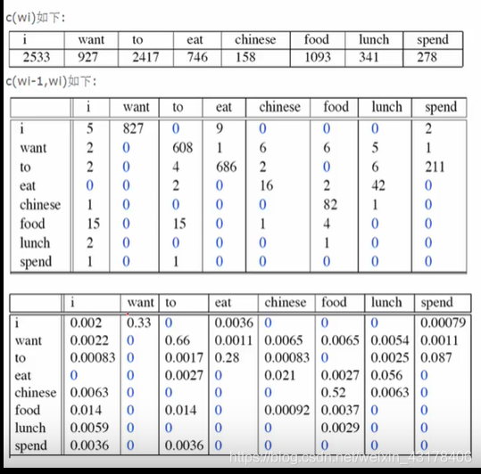
对于第二个表格，其意义是竖列中的单词出现后，横列单词出现的次数。那么如何从语料库得到上述表格？一般语料库是很多篇文档（个人认为如果一篇文档也很多句话，那么可以将每句话都当成一个独立的文档，后续所说文档指的是文档中的每句话），首先将文档进行分词。最终是类列表的结构，比如
[[the, cat, is, running],
[the, dog, is, cute, that, dog, is, smart]]
然后根据前面讲到的词袋进行统计单个单词出现的次数，两个单词出现的次数
现在假如我们现在要计算p(want|i):
$$p(want|i)=\frac{count(i,want)}{count(i)}=\frac{827}{2533}=0.33$$
对于一句话s = “I want food”，其计算公式为：
$$p(s)=p(I)p(want|I)p(food|want)$$
一般地，对于首个单词的概率p(I)我们认为$p(I)=p(I|<s>)$，其中$<s>$表示一篇文章的开始，此外$<e>$表示一篇文章的结束。因此$p(s)=p(I|<s>)p(want|I)p(food|want)p(<e>|food)$
对于$p(I)=p(I|<s>)$，上表中没有体现，现假设我们有10000篇文章，其中5000个文章的首个单词（除了$<s>$）都是以I开头的，那么$p(I)=p(I|<s>)=\frac{5000}{10000}=0.5$
对于$p(want|I)、p(food|want)$在表格中有体现，分别为0.33和0.0065。
对于$p(<e>|food)$在表格中也没有体现，假设我们10000篇文章中有100篇是以food结尾的，那么$p(<e>|food)=\frac{100}{10000}=0.01$
因此，最终：
$$p(s)=p(I|<s>)p(want|I)p(food|want)p(<e>|food)=0.5\ast 0.33\ast 0.0065\ast 0.01=1.0725e-5$$

如果一个词的出现与它周围的词是独立的，称为一元语言模型（unigram）；
如果一个词的出现仅依赖于它前面的一个词，称为二元语言模型（bigram）；
如果一个词的出现依赖于它前面的两个词，称为三元语言模型（trigram）；
其他的以此类推
下表是各种语言模型的参数量：

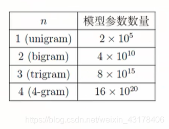
由此可见当n很大时，参数量也是很大的，一般我们用2-3即可。
关于语言模型的代码好像还没有进行封装，因此我们可以根据上述的CountVectorizer等自己写代码计算。语言模型更多的是理论，作为后续推出的各种模型的基础，如nnlm。

扫描二维码关注公众号，回复： 11945135 查看本文章

4.3.3 朴素贝叶斯模型&n-gram模型

上一小节讲到了n-gram，此n-garm是语言模型的一种假设，本小节所述n-garm以及贝叶斯是一种分类模型，具体详见博客https://blog.csdn.net/weixin_43178406/article/details/105702387

5. 词向量tf-idf

给定训练语料（corpus），如
[[the, cat, is, running],
[this, dog, is, cute, that, dog, is, smart]]
假如我们最终的词典为[‘cat’, ‘cute’, ‘dog’, ‘is’, ‘running’, ‘smart’, ‘that’, ‘the’, ‘this’]
那么the这个词经过tf-idf处理，就会得到一个对应的数字，词典中其他单词亦同。
那么这个数字是如何得到的？
tf-idf = tf × idf

1. 计算tf值，tf值就是词频，表示一个给定词语t在一篇给定文档d中出现的频率，即单词t出现的次数除以当前文档中词出现的总次数。tf越高，则词语t对文档d来说越重要，TF越低，则词语t对文档d来说越不重要。
2. 计算idf值：逆文档频率。tf值很高，并不能说明该词对文章的贡献度高，比如单词is在所有文章中出现的次数都很高，其tf值甚至高于关键词如doctor，但is并不是我们想要的（doctor才是）。所以此时需要计算一个逆文档频率。如is所有文档中出现次数都很高，那么出现该词的文章数除以所有文章数就越大，其倒数越小。因此用$log\frac{总文章数}{出现单词t的文章数}$来限制tf
3. 实际应用中，idf需要进行平滑处理，因为除数为0，就无法计算了。常用的平滑方法如下：
   $$log\frac{总文章数+1}{出现单词t的文章数+1}+1$$
   $$log\frac{总文章数}{出现单词t的文章数+1}$$

• 实例代码

# 使用sklearn中的TfidfVectorizor
from sklearn.feature_extraction.text import TfidfVectorizer
corpus = ['the cat is running',
         'this dog is cute, that dog is smart']
vectorizer = TfidfVectorizer()
X = vectorizer.fit_transform(corpus)
print(vectorizer.get_feature_names())
print(X.toarray())

['cat', 'cute', 'dog', 'is', 'running', 'smart', 'that', 'the', 'this']
[[0.53404633 0.         0.         0.37997836 0.53404633 0.
  0.         0.53404633 0.        ]
 [0.         0.3158336  0.6316672  0.44943642 0.         0.3158336
  0.3158336  0.         0.3158336 ]]

# 使用sklearn中的TfidfTransformer，与CountVectorizer搭配使用

# 先使用CountVectorizer
from sklearn.feature_extraction.text import CountVectorizer
corpus = ['the cat is running',
         'this dog is cute, that dog is smart']
vectorizer = CountVectorizer()
X = vectorizer.fit_transform(corpus)
print(vectorizer.get_feature_names())
print(X.toarray())

# 将X传入TfidfTransformer
from sklearn.feature_extraction.text import TfidfTransformer
idf = TfidfTransformer()
res = idf.fit_transform(X)  # 传入的X可以是稀疏矩阵，也可以是转换后的array
print(res.toarray())

['cat', 'cute', 'dog', 'is', 'running', 'smart', 'that', 'the', 'this']
[[1 0 0 1 1 0 0 1 0]
 [0 1 2 2 0 1 1 0 1]]
[[0.53404633 0.         0.         0.37997836 0.53404633 0.
  0.         0.53404633 0.        ]
 [0.         0.3158336  0.6316672  0.44943642 0.         0.3158336
  0.3158336  0.         0.3158336 ]]

可以发现TfidfVectorizer是TfidfTransformer和CountVectorizer的结合。因此TfidfVectorizer中的参数也是TfidfTransformer和CountVectorizer参数的结合。上文已经讲过CountVectorizer的参数了，现在详解TfidfTransformer的参数。

• use_idf：boolean，是否使用idf限制tf，如果为False，结果仅仅是tf
• smooth_idf：boolean，是否对idf加入平滑
  idf教科书公式$$log\frac{总文章数}{出现单词t的文章数+1}$$
  smooth_idf=True$$log\frac{总文章数+1}{出现单词t的文章数+1}+1$$
  smooth_idf=False$$log\frac{总文章数}{出现单词t的文章数}+1$$
• sublinear_tf：boolean，是否对tf进行转换。如果为False，tf计算的是词出现的次数，而不是词的频率，这一点和平时也不一样；如果为True,则tf为1+log(tf)，这里的tf仍然指词出现的次数
• norm：'l1’或’l2’或None。l1表示对计算出的tf-idf值进行l1范数的标准化；l2表示对计算出的tf-idf值进行l2范数的标准化；None不进行标准化。其中l1范数和l2范数都是对每一行，即每个文章
  l1范数公式$$v_{norm}=\frac{v}{||v|{|}_1}=\frac{v}{|v_1|+|v_2|+...+|v_n|}$$
  l2范数公式$$v_{norm}=\frac{v}{||v|{|}_1}=\frac{v}{(|v_1{|}^2+|v_2{|}^2+...+|v_n{|}^2{)}^{\frac{1}{2}}}$$

6. 词向量发展&语言模型

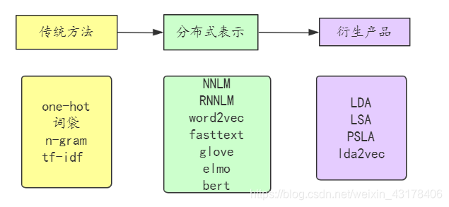
目前语言模型就是n-gram语言模型，有时，利用n-gram模型可以计算出副产品词向量
上述其他词向量可见其他博客