Tensorflow2.0 笔记

Tensorflow笔记

1 常用函数

1.1 tf.where()

import tensorflow as tf

a = tf.constant([1, 2, 3, 1, 1])
b = tf.constant([0, 1, 3, 4, 5])
c = tf.where(tf.greater(a, b), a, b)  # 若a>b，返回a对应位置的元素，否则返回b对应位置的元素
print("c：", c)

c： tf.Tensor([1 2 3 4 5], shape=(5,), dtype=int32)

1.2 np.mgrid()

import numpy as np
import tensorflow as tf

# 生成等间隔数值点
x, y = np.mgrid[1:3:1, 2:4:0.5]
# 将x, y拉直，并合并配对为二维张量，生成二维坐标点
grid = np.c_[x.ravel(), y.ravel()]

print("x:\n", x)
print("y:\n", y)
print("x.ravel():\n", x.ravel())
print("y.ravel():\n", y.ravel())
print('grid:\n', grid)

x:
[[1. 1. 1. 1.]
[2. 2. 2. 2.]]
y:
[[2. 2.5 3. 3.5]
[2. 2.5 3. 3.5]]

x.ravel():
[1. 1. 1. 1. 2. 2. 2. 2.]
y.ravel():
[2. 2.5 3. 3.5 2. 2.5 3. 3.5]

grid:
[[1. 2. ]
[1. 2.5]
[1. 3. ]
[1. 3.5]
[2. 2. ]
[2. 2.5]
[2. 3. ]
[2. 3.5]]

1.3 tf.nn.softmax_cross_entropy_with_logits()

# softmax与交叉熵损失函数的结合
import tensorflow as tf
import numpy as np

y_ = np.array([[1, 0, 0], [0, 1, 0], [0, 0, 1], [1, 0, 0], [0, 1, 0]])
y = np.array([[12, 3, 2], [3, 10, 1], [1, 2, 5], [4, 6.5, 1.2], [3, 6, 1]])

y_pro = tf.nn.softmax(y)                                    # 1
loss_ce1 = tf.losses.categorical_crossentropy(y_,y_pro)     # 2

loss_ce2 = tf.nn.softmax_cross_entropy_with_logits(y_, y)   # 3,把1和2结合起来，用这一行代替两行

print('分步计算的结果:\n', loss_ce1)
print('结合计算的结果:\n', loss_ce2)

# 输出的结果相同

2 常用网络的代码实现

本节按网络的复杂程度进行内容编写。

2.1 基础框架——Sequential 和 Class 网络框架

使用Mnist数据集。下面给出最基本的框架样例。

2.1.1 tf.keras.models.Sequential()

import tensorflow as tf

mnist = tf.keras.datasets.mnist
(x_train, y_train), (x_test, y_test) = mnist.load_data()
x_train, x_test = x_train / 255.0, x_test / 255.0

model = tf.keras.models.Sequential([
    tf.keras.layers.Flatten(),
    tf.keras.layers.Dense(128, activation='relu'),
    tf.keras.layers.Dense(10, activation='softmax')
])

model.compile(optimizer='adam',
              loss=tf.keras.losses.SparseCategoricalCrossentropy(from_logits=False),
              metrics=['sparse_categorical_accuracy'])

model.fit(x_train, y_train, batch_size=32, epochs=5, validation_data=(x_test, y_test), validation_freq=1)
model.summary()

2.1.2 class MyModel (Model)

import tensorflow as tf
from tensorflow.keras.layers import Dense, Flatten
from tensorflow.keras import Model

mnist = tf.keras.datasets.mnist
(x_train, y_train), (x_test, y_test) = mnist.load_data()
x_train, x_test = x_train / 255.0, x_test / 255.0


class MnistModel(Model):
    def __init__(self):
        super(MnistModel, self).__init__()
        self.flatten = Flatten()
        self.d1 = Dense(128, activation='relu')
        self.d2 = Dense(10, activation='softmax')

    def call(self, x):
        x = self.flatten(x)
        x = self.d1(x)
        y = self.d2(x)
        return y


model = MnistModel()

model.compile(optimizer='adam',
              loss=tf.keras.losses.SparseCategoricalCrossentropy(from_logits=False),
              metrics=['sparse_categorical_accuracy'])

model.fit(x_train, y_train, batch_size=32, epochs=5, validation_data=(x_test, y_test), validation_freq=1)
model.summary()

2.2 功能扩展后的网络

2.2.1 构造数据集

标签文件格式如下所示：

文件名 标签

1_9.jpg 9
2_0.jpg 0
3_0.jpg 0
4_3.jpg 3
5_0.jpg 0
6_2.jpg 2
7_7.jpg 7
8_2.jpg 2
9_5.jpg 5
10_5.jpg 5

import tensorflow as tf
from PIL import Image
import numpy as np
import os

train_path = './fashion_image_label/fashion_train_jpg_60000/'
train_txt = './fashion_image_label/fashion_train_jpg_60000.txt'
x_train_savepath = './fashion_image_label/fashion_x_train.npy'
y_train_savepath = './fashion_image_label/fahion_y_train.npy'

test_path = './fashion_image_label/fashion_test_jpg_10000/'
test_txt = './fashion_image_label/fashion_test_jpg_10000.txt'
x_test_savepath = './fashion_image_label/fashion_x_test.npy'
y_test_savepath = './fashion_image_label/fashion_y_test.npy'


def generateds(path, txt):
    f = open(txt, 'r')
    contents = f.readlines()  # 按行读取
    f.close()
    x, y_ = [], []
    for content in contents:
        value = content.split()  # 以空格分开，存入数组
        img_path = path + value[0]
        img = Image.open(img_path)
        img = np.array(img.convert('L'))
        img = img / 255.
        x.append(img)
        y_.append(value[1])
        print('loading : ' + content)

    x = np.array(x)
    y_ = np.array(y_)
    y_ = y_.astype(np.int64)
    return x, y_


if os.path.exists(x_train_savepath) and os.path.exists(y_train_savepath) and os.path.exists(
        x_test_savepath) and os.path.exists(y_test_savepath):
    print('-------------Load Datasets-----------------')
    x_train_save = np.load(x_train_savepath)
    y_train = np.load(y_train_savepath)
    x_test_save = np.load(x_test_savepath)
    y_test = np.load(y_test_savepath)
    x_train = np.reshape(x_train_save, (len(x_train_save), 28, 28))
    x_test = np.reshape(x_test_save, (len(x_test_save), 28, 28))
else:
    print('-------------Generate Datasets-----------------')
    x_train, y_train = generateds(train_path, train_txt) # generaterds 的返回值应该就是（28，28）的，所以下面的 x_train_save
                                                         # 就变成了（-1），应该是这样保存更省空间吧？
    x_test, y_test = generateds(test_path, test_txt)

    print('-------------Save Datasets-----------------')
    x_train_save = np.reshape(x_train, (len(x_train), -1))
    x_test_save = np.reshape(x_test, (len(x_test), -1))
    np.save(x_train_savepath, x_train_save)
    np.save(y_train_savepath, y_train)
    np.save(x_test_savepath, x_test_save)
    np.save(y_test_savepath, y_test)

model = tf.keras.models.Sequential([
    tf.keras.layers.Flatten(),
    tf.keras.layers.Dense(128, activation='relu'),
    tf.keras.layers.Dense(10, activation='softmax')
])

model.compile(optimizer='adam',
              loss=tf.keras.losses.SparseCategoricalCrossentropy(from_logits=False),
              metrics=['sparse_categorical_accuracy'])

model.fit(x_train, y_train, batch_size=32, epochs=5, validation_data=(x_test, y_test), validation_freq=1)
model.summary()

2.2.2 图片数据增强

# 显示原始图像和增强后的图像
import tensorflow as tf
from matplotlib import pyplot as plt
from tensorflow.keras.preprocessing.image import ImageDataGenerator
import numpy as np

mnist = tf.keras.datasets.fashion_mnist
(x_train, y_train), (x_test, y_test) = mnist.load_data()
x_train = x_train.reshape(x_train.shape[0], 28, 28, 1) # 1：通道个数为 1
x_test = x_test.reshape(x_test.shape[0], 28, 28, 1)

image_gen_train = ImageDataGenerator(
    rescale=1. / 255,       # 所有数据将乘以该数值
    rotation_range=45,      # 随机旋转角度数范围
    width_shift_range=.15,  # 随机宽度偏移量
    height_shift_range=.15, # 随机高度偏移量
    horizontal_flip=True,   # 是否随机水平翻转
    zoom_range=0.5          # 随机缩放的范围 [1-n，1+n]
)
image_gen_train.fit(x_train)

x_train_subset1 = np.squeeze(x_train[:12]) # np.squeeze()把维度是1的去掉。在这里是把通道那个维度去掉了
x_train_subset2 = x_train[:12]  # 一次显示12张图片。下面image_gen_train.flow()需要用到通道，所以这里不使用np.squeeze()

fig = plt.figure(figsize=(20, 2))
plt.set_cmap('gray')
# 显示原始图片
for i in range(0, len(x_train_subset1)):
    ax = fig.add_subplot(1, 12, i + 1)
    ax.imshow(x_train_subset1[i])
fig.suptitle('Subset of Original Training Images', fontsize=20)
plt.show()

# 显示增强后的图片
fig = plt.figure(figsize=(20, 2))
# 第一个for循环就是这么写的
for x_batch in image_gen_train.flow(x_train_subset2, batch_size=12, shuffle=False):
    for i in range(0, 12):
        ax = fig.add_subplot(1, 12, i + 1)
        ax.imshow(np.squeeze(x_batch[i])) # 维度为1的去掉，在这里去掉了通道
    fig.suptitle('Augmented Images', fontsize=20)
    plt.show()
    break

2.2.3 断点续训、输出网络参数、输出loss曲线

import tensorflow as tf
import os
import numpy as np
from matplotlib import pyplot as plt

## 可以打印出无限条内容
np.set_printoptions(threshold=np.inf)

## 加载数据集
fashion = tf.keras.datasets.fashion_mnist
(x_train, y_train), (x_test, y_test) = fashion.load_data()
x_train, x_test = x_train / 255.0, x_test / 255.0

## 定义网络结构
model = tf.keras.models.Sequential([
    tf.keras.layers.Flatten(),
    tf.keras.layers.Dense(128, activation='relu'),
    tf.keras.layers.Dense(10, activation='softmax')
])

## 神经网络优化
model.compile(optimizer='adam',
              loss=tf.keras.losses.SparseCategoricalCrossentropy(from_logits=False),
              metrics=['sparse_categorical_accuracy'])

## 保存已训练的模型
# 路径
checkpoint_save_path = "./checkpoint/fashion.ckpt"
# 加载已保存的模型
if os.path.exists(checkpoint_save_path + '.index'):
    print('-------------load the model-----------------')
    model.load_weights(checkpoint_save_path)

cp_callback = tf.keras.callbacks.ModelCheckpoint(filepath=checkpoint_save_path,
                                                 save_weights_only=True,
                                                 save_best_only=True)
## 训练
history = model.fit(x_train, y_train,
                    batch_size=32, 
                    epochs=5, 
                    validation_data=(x_test, y_test), 
                    validation_freq=1,
                    callbacks=[cp_callback]
                   )

## 打印网络结构
model.summary()

## 打印网络参数并保存为txt文件
print(model.trainable_variables)
file = open('./weights.txt', 'w')
for v in model.trainable_variables:
    file.write(str(v.name) + '\n')
    file.write(str(v.shape) + '\n')
    file.write(str(v.numpy()) + '\n') # ???????????????
file.close()

## 显示训练集和验证集的acc和loss曲线
# 训练集acc
acc = history.history['sparse_categorical_accuracy']
# 测试集acc
val_acc = history.history['val_sparse_categorical_accuracy']
# 训练误差
loss = history.history['loss']
# 测试误差
val_loss = history.history['val_loss']

## 输出误差下降曲线
# 子图1
plt.subplot(1, 2, 1)
plt.plot(acc, label='Training Accuracy')
plt.plot(val_acc, label='Validation Accuracy')
plt.title('Training and Validation Accuracy')
plt.legend()

# 子图2
plt.subplot(1, 2, 2)
plt.plot(loss, label='Training Loss')
plt.plot(val_loss, label='Validation Loss')
plt.title('Training and Validation Loss')
plt.legend()

plt.show()

2.2.4 手写数字识别——model.predict()

from PIL import Image
import numpy as np
import tensorflow as tf
import matplotlib.pyplot as plt
type = ['T-shirt/top', 'Trouser', 'Pullover', 'Dress', 'Coat', 'Sandal', 'Shirt', 'Sneaker', 'Bag', 'Ankle boot']

model_save_path = './checkpoint/fashion.ckpt'
model = tf.keras.models.Sequential([
    tf.keras.layers.Flatten(),
    tf.keras.layers.Dense(128, activation='relu'),
    tf.keras.layers.Dense(10, activation='softmax')
])
                                        
model.load_weights(model_save_path)

preNum = int(input("input the number of test pictures:"))
for i in range(preNum):
    image_path = input("the path of test picture:")
    img = Image.open(image_path)
    image = plt.imread(image_path)
    plt.set_cmap('gray') # 转化成灰度图
    plt.imshow(image)

    img=img.resize((28,28),Image.ANTIALIAS) # Image.ANTIALIAS：反锯齿过滤器
    img_arr = np.array(img.convert('L'))
    img_arr = 255 - img_arr #每个像素点= 255 - 各自点当前灰度值。从黑底白字变成了白底黑字

    img_arr=img_arr/255.0 # 归一化

    x_predict = img_arr[tf.newaxis,...] # 增加一个维度，表示 1 张维度为(28，28)的图片

    result = model.predict(x_predict)
    pred=tf.argmax(result, axis=1)
    print('\n')
    print(type[int(pred)])

    plt.pause(1)
    plt.close()

2.3 卷积神经网络

卷积神经网络：借助卷积核提取特征后，送入全连接网络。

• 框架

2.3.1 卷积——特征提取器

实际应用时会先对原始图像进行特征提取再把提取到的特征送给全连接网络。

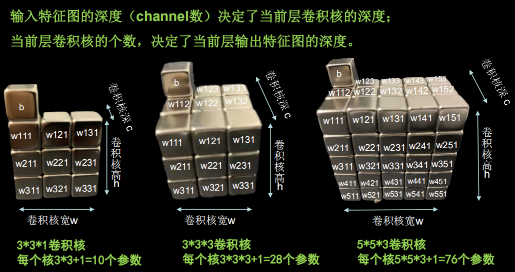
• 卷积核
  1. 一般用两个3*3的卷积核代替一个5*5的卷积核，因为这样子计算量会减小
  2. 若是三通道的图片，那么需要深度为3的卷积核（三个卷积核）

▲ 不同类型的卷积核

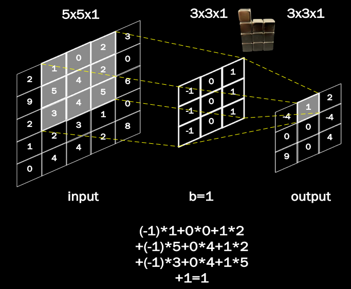
• 卷积的计算

• 感受野
  

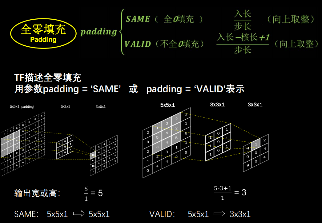
• 全零填充
  

2.3.2 卷积层的Tensorflow表示

tf.keras.layers.Conv2D (
	filters = 卷积核个数, 
	kernel_size = 卷积核尺寸, #正方形写核长整数，或（核高h，核宽w）
	strides = 滑动步长, #横纵向相同写步长整数，或(纵向步长h，横向步长w)，默认1
	padding = “same” or “valid”, #使用全零填充是“same”，不使用是“valid”（默认）
	activation = “ relu ” or “ sigmoid ” or “ tanh ” or “ softmax”等 , #如有BN此处不写
	input_shape = (高, 宽 , 通道数) #输入特征图维度，可省略
)

在网络中卷积层的三种定义方式：

model = tf.keras.models.Sequential([
	Conv2D(6, 5, padding='valid', activation='sigmoid'), 	  # 1
	MaxPool2D(2, 2),
	Conv2D(6, (5, 5), padding='valid', activation='sigmoid'), # 2
	MaxPool2D(2, (2, 2)),
	Conv2D(filters=6, kernel_size=(5, 5),padding='valid', activation='sigmoid'), # 3
	MaxPool2D(pool_size=(2, 2), strides=2),
	Flatten(),
	Dense(10, activation='softmax')
])

推荐第三种表达方式，代码可读性较高。

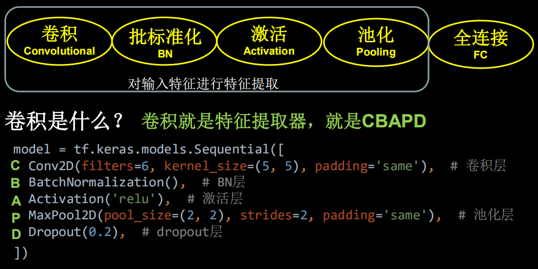
2.3.3 批标准化 （Batch Normalization， BN）

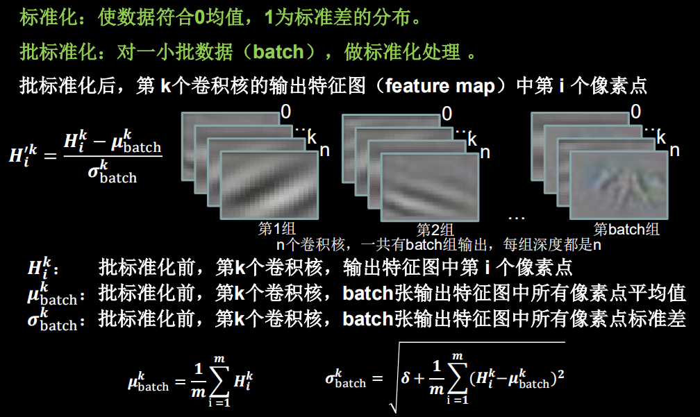
• BN层位于卷积层之后，激活层之前。

2.3.3 批标准化的Tensorflow表示

tf.keras.layers.BatchNormalization()

model = tf.keras.models.Sequential([
	Conv2D(filters=6, kernel_size=(5, 5), padding='same'), # 卷积层
	BatchNormalization(), # BN层
	Activation('relu'), # 激活层
	MaxPool2D(pool_size=(2, 2), strides=2, padding='same'), # 池化层
	Dropout(0.2), # dropout层
])

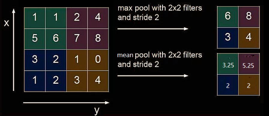
2.3.4 池化（pooling）

池化用于减少特征数据量。
最大值池化可提取图片纹理，均值池化可保留背景特征。

2.3.5 池化层的Tensorflow表示

# 最大池化
tf.keras.layers.MaxPool2D(
	pool_size=池化核尺寸，#正方形写核长整数，或（核高h，核宽w）
	strides=池化步长，#步长整数， 或(纵向步长h，横向步长w)，默认为pool_size
	padding=‘valid’or‘same’ #使用全零填充是“same”，不使用是“valid”（默认）
)
# 平均池化
tf.keras.layers.AveragePooling2D(
	pool_size=池化核尺寸，#正方形写核长整数，或（核高h，核宽w）
	strides=池化步长，#步长整数， 或(纵向步长h，横向步长w)，默认为pool_size
	padding=‘valid’or‘same’ #使用全零填充是“same”，不使用是“valid”（默认）
)

# 应用于网咯中
model = tf.keras.models.Sequential([
	Conv2D(filters=6, kernel_size=(5, 5), padding='same'), # 卷积层
	BatchNormalization(), # BN层
	Activation('relu'), # 激活层
	MaxPool2D(pool_size=(2, 2), strides=2, padding='same'), # 池化层
	Dropout(0.2), # dropout层
])

2.3.6 舍弃（dropout）

在神经网络训练时，将一部分神经元按照一定概率从神经网络中暂时舍弃。神经网络使用时，被舍弃的神经元恢复链接。

tf.keras.layers.Dropout(舍弃的概率)

model = tf.keras.models.Sequential([
	Conv2D(filters=6, kernel_size=(5, 5), padding='same'), # 卷积层
	BatchNormalization(), # BN层
	Activation('relu'), # 激活层
	MaxPool2D(pool_size=(2, 2), strides=2, padding='same'), # 池化层
	Dropout(0.2), # dropout层
])

2.3.7 完整的卷积神经网络——“CBAPD”

代码：

import tensorflow as tf
import os
import numpy as np
from matplotlib import pyplot as plt
from tensorflow.keras.layers import Conv2D, BatchNormalization, Activation, MaxPool2D, Dropout, Flatten, Dense
from tensorflow.keras import Model

np.set_printoptions(threshold=np.inf)

cifar10 = tf.keras.datasets.cifar10
(x_train, y_train), (x_test, y_test) = cifar10.load_data()
x_train, x_test = x_train / 255.0, x_test / 255.0


class Baseline(Model):
    def __init__(self):
        super(Baseline, self).__init__()
        self.c1 = Conv2D(filters=6, kernel_size=(5, 5), padding='same')  # 卷积层
        self.b1 = BatchNormalization()  # BN层
        self.a1 = Activation('relu')  # 激活层
        self.p1 = MaxPool2D(pool_size=(2, 2), strides=2, padding='same')  # 池化层
        self.d1 = Dropout(0.2)  # dropout层

        self.flatten = Flatten()
        self.f1 = Dense(128, activation='relu')
        self.d2 = Dropout(0.2)
        self.f2 = Dense(10, activation='softmax')

    def call(self, x):
        x = self.c1(x)
        x = self.b1(x)
        x = self.a1(x)
        x = self.p1(x)
        x = self.d1(x)

        x = self.flatten(x)
        x = self.f1(x)
        x = self.d2(x)
        y = self.f2(x)
        return y


model = Baseline()

model.compile(optimizer='adam',
              loss=tf.keras.losses.SparseCategoricalCrossentropy(from_logits=False),
              metrics=['sparse_categorical_accuracy'])

checkpoint_save_path = "./checkpoint/Baseline.ckpt"
if os.path.exists(checkpoint_save_path + '.index'):
    print('-------------load the model-----------------')
    model.load_weights(checkpoint_save_path)

cp_callback = tf.keras.callbacks.ModelCheckpoint(filepath=checkpoint_save_path,
                                                 save_weights_only=True,
                                                 save_best_only=True)

history = model.fit(x_train, y_train, batch_size=32, epochs=5, validation_data=(x_test, y_test), validation_freq=1,
                    callbacks=[cp_callback])
model.summary()

# print(model.trainable_variables)
file = open('./weights.txt', 'w')
for v in model.trainable_variables:
    file.write(str(v.name) + '\n')
    file.write(str(v.shape) + '\n')
    file.write(str(v.numpy()) + '\n')
file.close()

###############################################    show   ###############################################

# 显示训练集和验证集的acc和loss曲线
acc = history.history['sparse_categorical_accuracy']
val_acc = history.history['val_sparse_categorical_accuracy']
loss = history.history['loss']
val_loss = history.history['val_loss']

plt.subplot(1, 2, 1)
plt.plot(acc, label='Training Accuracy')
plt.plot(val_acc, label='Validation Accuracy')
plt.title('Training and Validation Accuracy')
plt.legend()

plt.subplot(1, 2, 2)
plt.plot(loss, label='Training Loss')
plt.plot(val_loss, label='Validation Loss')
plt.title('Training and Validation Loss')
plt.legend()
plt.show()

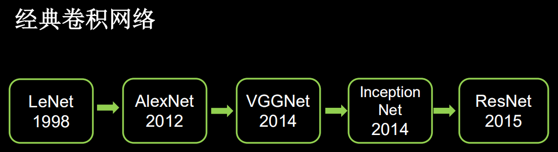
2.4 常见的经典卷积神经网络

以下代码均使用cifar10数据集。
本节按各卷积神经网络出现的时间顺序编写。

Tips：

1. 编写神经网络的时候，可以先把它的框架结构表示出来，然后再根据框架编写代码。
2. 牢记"CBAPD"卷积神经网络结构。

2.4.1 加载cifar10数据集

import tensorflow as tf
from matplotlib import pyplot as plt
import numpy as np

np.set_printoptions(threshold=np.inf)

cifar10 = tf.keras.datasets.cifar10
(x_train, y_train), (x_test, y_test) = cifar10.load_data()

# 可视化训练集输入特征的第一个元素
plt.imshow(x_train[0])  # 绘制图片
plt.show()

# 打印出训练集输入特征的第一个元素
print("x_train[0]:\n", x_train[0])
# 打印出训练集标签的第一个元素
print("y_train[0]:\n", y_train[0])

# 打印出整个训练集输入特征形状
print("x_train.shape:\n", x_train.shape)
# 打印出整个训练集标签的形状
print("y_train.shape:\n", y_train.shape)
# 打印出整个测试集输入特征的形状
print("x_test.shape:\n", x_test.shape)
# 打印出整个测试集标签的形状
print("y_test.shape:\n", y_test.shape)

2.4.1 baseline

各卷积神经网络的基础框架，不同的卷积神经网络的网络结构部分不同。

import tensorflow as tf
import os
import numpy as np
from matplotlib import pyplot as plt
from tensorflow.keras.layers import Conv2D, BatchNormalization, Activation, MaxPool2D, Dropout, Flatten, Dense
from tensorflow.keras import Model

np.set_printoptions(threshold=np.inf)

cifar10 = tf.keras.datasets.cifar10
(x_train, y_train), (x_test, y_test) = cifar10.load_data()
x_train, x_test = x_train / 255.0, x_test / 255.0


class Baseline(Model):
    def __init__(self):
        super(Baseline, self).__init__()
        self.c1 = Conv2D(filters=6, kernel_size=(5, 5), padding='same')  # 卷积层
        self.b1 = BatchNormalization()  # BN层
        self.a1 = Activation('relu')  # 激活层
        self.p1 = MaxPool2D(pool_size=(2, 2), strides=2, padding='same')  # 池化层
        self.d1 = Dropout(0.2)  # dropout层

        self.flatten = Flatten()
        self.f1 = Dense(128, activation='relu')
        self.d2 = Dropout(0.2)
        self.f2 = Dense(10, activation='softmax')

    def call(self, x):
        x = self.c1(x)
        x = self.b1(x)
        x = self.a1(x)
        x = self.p1(x)
        x = self.d1(x)

        x = self.flatten(x)
        x = self.f1(x)
        x = self.d2(x)
        y = self.f2(x)
        return y


model = Baseline()

model.compile(optimizer='adam',
              loss=tf.keras.losses.SparseCategoricalCrossentropy(from_logits=False),
              metrics=['sparse_categorical_accuracy'])

checkpoint_save_path = "./checkpoint/Baseline.ckpt"
if os.path.exists(checkpoint_save_path + '.index'):
    print('-------------load the model-----------------')
    model.load_weights(checkpoint_save_path)

cp_callback = tf.keras.callbacks.ModelCheckpoint(filepath=checkpoint_save_path,
                                                 save_weights_only=True,
                                                 save_best_only=True)

history = model.fit(x_train, y_train, batch_size=32, epochs=5, validation_data=(x_test, y_test), validation_freq=1,
                    callbacks=[cp_callback])
model.summary()

# print(model.trainable_variables)
file = open('./weights.txt', 'w')
for v in model.trainable_variables:
    file.write(str(v.name) + '\n')
    file.write(str(v.shape) + '\n')
    file.write(str(v.numpy()) + '\n')
file.close()

###############################################    show   ###############################################

# 显示训练集和验证集的acc和loss曲线
acc = history.history['sparse_categorical_accuracy']
val_acc = history.history['val_sparse_categorical_accuracy']
loss = history.history['loss']
val_loss = history.history['val_loss']

plt.subplot(1, 2, 1)
plt.plot(acc, label='Training Accuracy')
plt.plot(val_acc, label='Validation Accuracy')
plt.title('Training and Validation Accuracy')
plt.legend()

plt.subplot(1, 2, 2)
plt.plot(loss, label='Training Loss')
plt.plot(val_loss, label='Validation Loss')
plt.title('Training and Validation Loss')
plt.legend()
plt.show()

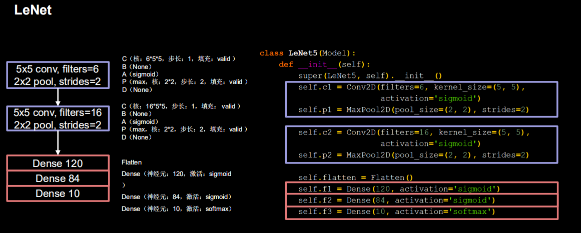
2.4.3 LeNet5

import tensorflow as tf
import os
import numpy as np
from matplotlib import pyplot as plt
from tensorflow.keras.layers import Conv2D, BatchNormalization, Activation, MaxPool2D, Dropout, Flatten, Dense
from tensorflow.keras import Model

np.set_printoptions(threshold=np.inf)

cifar10 = tf.keras.datasets.cifar10
(x_train, y_train), (x_test, y_test) = cifar10.load_data()
x_train, x_test = x_train / 255.0, x_test / 255.0


class LeNet5(Model):
    def __init__(self):
        super(LeNet5, self).__init__()
        self.c1 = Conv2D(filters=6, kernel_size=(5, 5),
                         activation='sigmoid')
        self.p1 = MaxPool2D(pool_size=(2, 2), strides=2)

        self.c2 = Conv2D(filters=16, kernel_size=(5, 5),
                         activation='sigmoid')
        self.p2 = MaxPool2D(pool_size=(2, 2), strides=2)

        self.flatten = Flatten()
        self.f1 = Dense(120, activation='sigmoid')
        self.f2 = Dense(84, activation='sigmoid')
        self.f3 = Dense(10, activation='softmax')

    def call(self, x):
        x = self.c1(x)
        x = self.p1(x)

        x = self.c2(x)
        x = self.p2(x)

        x = self.flatten(x)
        x = self.f1(x)
        x = self.f2(x)
        y = self.f3(x)
        return y


model = LeNet5()

model.compile(optimizer='adam',
              loss=tf.keras.losses.SparseCategoricalCrossentropy(from_logits=False),
              metrics=['sparse_categorical_accuracy'])

checkpoint_save_path = "./checkpoint/LeNet5.ckpt"
if os.path.exists(checkpoint_save_path + '.index'):
    print('-------------load the model-----------------')
    model.load_weights(checkpoint_save_path)

cp_callback = tf.keras.callbacks.ModelCheckpoint(filepath=checkpoint_save_path,
                                                 save_weights_only=True,
                                                 save_best_only=True)

history = model.fit(x_train, y_train, batch_size=32, epochs=5, validation_data=(x_test, y_test), validation_freq=1,
                    callbacks=[cp_callback])
model.summary()

# print(model.trainable_variables)
file = open('./weights.txt', 'w')
for v in model.trainable_variables:
    file.write(str(v.name) + '\n')
    file.write(str(v.shape) + '\n')
    file.write(str(v.numpy()) + '\n')
file.close()

###############################################    show   ###############################################

# 显示训练集和验证集的acc和loss曲线
acc = history.history['sparse_categorical_accuracy']
val_acc = history.history['val_sparse_categorical_accuracy']
loss = history.history['loss']
val_loss = history.history['val_loss']

plt.subplot(1, 2, 1)
plt.plot(acc, label='Training Accuracy')
plt.plot(val_acc, label='Validation Accuracy')
plt.title('Training and Validation Accuracy')
plt.legend()

plt.subplot(1, 2, 2)
plt.plot(loss, label='Training Loss')
plt.plot(val_loss, label='Validation Loss')
plt.title('Training and Validation Loss')
plt.legend()
plt.show()

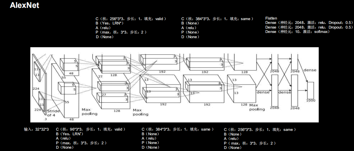
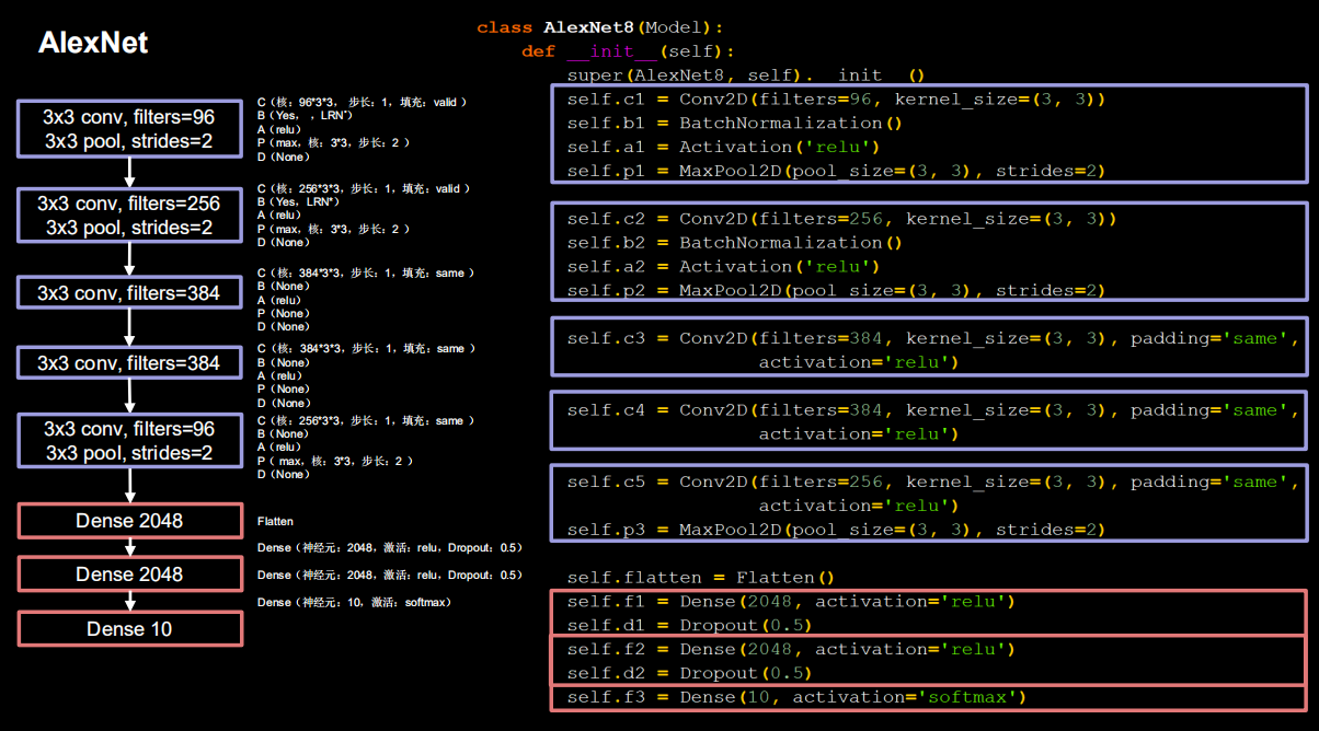
2.4.4 AlexNet8

import tensorflow as tf
import os
import numpy as np
from matplotlib import pyplot as plt
from tensorflow.keras.layers import Conv2D, BatchNormalization, Activation, MaxPool2D, Dropout, Flatten, Dense
from tensorflow.keras import Model

np.set_printoptions(threshold=np.inf)

cifar10 = tf.keras.datasets.cifar10
(x_train, y_train), (x_test, y_test) = cifar10.load_data()
x_train, x_test = x_train / 255.0, x_test / 255.0


class AlexNet8(Model):
    def __init__(self):
        super(AlexNet8, self).__init__()
        self.c1 = Conv2D(filters=96, kernel_size=(3, 3))
        self.b1 = BatchNormalization()
        self.a1 = Activation('relu')
        self.p1 = MaxPool2D(pool_size=(3, 3), strides=2)

        self.c2 = Conv2D(filters=256, kernel_size=(3, 3))
        self.b2 = BatchNormalization()
        self.a2 = Activation('relu')
        self.p2 = MaxPool2D(pool_size=(3, 3), strides=2)

        self.c3 = Conv2D(filters=384, kernel_size=(3, 3), padding='same',
                         activation='relu')
                         
        self.c4 = Conv2D(filters=384, kernel_size=(3, 3), padding='same',
                         activation='relu')
                         
        self.c5 = Conv2D(filters=256, kernel_size=(3, 3), padding='same',
                         activation='relu')
        self.p3 = MaxPool2D(pool_size=(3, 3), strides=2)

        self.flatten = Flatten()
        self.f1 = Dense(2048, activation='relu')
        self.d1 = Dropout(0.5)
        self.f2 = Dense(2048, activation='relu')
        self.d2 = Dropout(0.5)
        self.f3 = Dense(10, activation='softmax')

    def call(self, x):
        x = self.c1(x)
        x = self.b1(x)
        x = self.a1(x)
        x = self.p1(x)

        x = self.c2(x)
        x = self.b2(x)
        x = self.a2(x)
        x = self.p2(x)

        x = self.c3(x)

        x = self.c4(x)

        x = self.c5(x)
        x = self.p3(x)

        x = self.flatten(x)
        x = self.f1(x)
        x = self.d1(x)
        x = self.f2(x)
        x = self.d2(x)
        y = self.f3(x)
        return y


model = AlexNet8()

model.compile(optimizer='adam',
              loss=tf.keras.losses.SparseCategoricalCrossentropy(from_logits=False),
              metrics=['sparse_categorical_accuracy'])

checkpoint_save_path = "./checkpoint/AlexNet8.ckpt"
if os.path.exists(checkpoint_save_path + '.index'):
    print('-------------load the model-----------------')
    model.load_weights(checkpoint_save_path)

cp_callback = tf.keras.callbacks.ModelCheckpoint(filepath=checkpoint_save_path,
                                                 save_weights_only=True,
                                                 save_best_only=True)

history = model.fit(x_train, y_train, batch_size=32, epochs=5, validation_data=(x_test, y_test), validation_freq=1,
                    callbacks=[cp_callback])
model.summary()

# print(model.trainable_variables)
file = open('./weights.txt', 'w')
for v in model.trainable_variables:
    file.write(str(v.name) + '\n')
    file.write(str(v.shape) + '\n')
    file.write(str(v.numpy()) + '\n')
file.close()

###############################################    show   ###############################################

# 显示训练集和验证集的acc和loss曲线
acc = history.history['sparse_categorical_accuracy']
val_acc = history.history['val_sparse_categorical_accuracy']
loss = history.history['loss']
val_loss = history.history['val_loss']

plt.subplot(1, 2, 1)
plt.plot(acc, label='Training Accuracy')
plt.plot(val_acc, label='Validation Accuracy')
plt.title('Training and Validation Accuracy')
plt.legend()

plt.subplot(1, 2, 2)
plt.plot(loss, label='Training Loss')
plt.plot(val_loss, label='Validation Loss')
plt.title('Training and Validation Loss')
plt.legend()
plt.show()

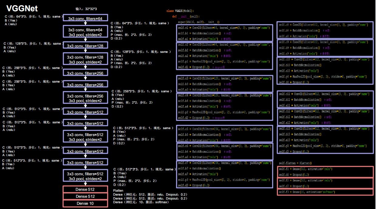
2.4.5 VGGNet16

import tensorflow as tf
import os
import numpy as np
from matplotlib import pyplot as plt
from tensorflow.keras.layers import Conv2D, BatchNormalization, Activation, MaxPool2D, Dropout, Flatten, Dense
from tensorflow.keras import Model

np.set_printoptions(threshold=np.inf)

cifar10 = tf.keras.datasets.cifar10
(x_train, y_train), (x_test, y_test) = cifar10.load_data()
x_train, x_test = x_train / 255.0, x_test / 255.0


class VGG16(Model):
    def __init__(self):
        super(VGG16, self).__init__()
        self.c1 = Conv2D(filters=64, kernel_size=(3, 3), padding='same')  # 卷积层1
        self.b1 = BatchNormalization()  # BN层1
        self.a1 = Activation('relu')  # 激活层1
        self.c2 = Conv2D(filters=64, kernel_size=(3, 3), padding='same', )
        self.b2 = BatchNormalization()  # BN层1
        self.a2 = Activation('relu')  # 激活层1
        self.p1 = MaxPool2D(pool_size=(2, 2), strides=2, padding='same')
        self.d1 = Dropout(0.2)  # dropout层

        self.c3 = Conv2D(filters=128, kernel_size=(3, 3), padding='same')
        self.b3 = BatchNormalization()  # BN层1
        self.a3 = Activation('relu')  # 激活层1
        self.c4 = Conv2D(filters=128, kernel_size=(3, 3), padding='same')
        self.b4 = BatchNormalization()  # BN层1
        self.a4 = Activation('relu')  # 激活层1
        self.p2 = MaxPool2D(pool_size=(2, 2), strides=2, padding='same')
        self.d2 = Dropout(0.2)  # dropout层

        self.c5 = Conv2D(filters=256, kernel_size=(3, 3), padding='same')
        self.b5 = BatchNormalization()  # BN层1
        self.a5 = Activation('relu')  # 激活层1
        self.c6 = Conv2D(filters=256, kernel_size=(3, 3), padding='same')
        self.b6 = BatchNormalization()  # BN层1
        self.a6 = Activation('relu')  # 激活层1
        self.c7 = Conv2D(filters=256, kernel_size=(3, 3), padding='same')
        self.b7 = BatchNormalization()
        self.a7 = Activation('relu')
        self.p3 = MaxPool2D(pool_size=(2, 2), strides=2, padding='same')
        self.d3 = Dropout(0.2)

        self.c8 = Conv2D(filters=512, kernel_size=(3, 3), padding='same')
        self.b8 = BatchNormalization()  # BN层1
        self.a8 = Activation('relu')  # 激活层1
        self.c9 = Conv2D(filters=512, kernel_size=(3, 3), padding='same')
        self.b9 = BatchNormalization()  # BN层1
        self.a9 = Activation('relu')  # 激活层1
        self.c10 = Conv2D(filters=512, kernel_size=(3, 3), padding='same')
        self.b10 = BatchNormalization()
        self.a10 = Activation('relu')
        self.p4 = MaxPool2D(pool_size=(2, 2), strides=2, padding='same')
        self.d4 = Dropout(0.2)

        self.c11 = Conv2D(filters=512, kernel_size=(3, 3), padding='same')
        self.b11 = BatchNormalization()  # BN层1
        self.a11 = Activation('relu')  # 激活层1
        self.c12 = Conv2D(filters=512, kernel_size=(3, 3), padding='same')
        self.b12 = BatchNormalization()  # BN层1
        self.a12 = Activation('relu')  # 激活层1
        self.c13 = Conv2D(filters=512, kernel_size=(3, 3), padding='same')
        self.b13 = BatchNormalization()
        self.a13 = Activation('relu')
        self.p5 = MaxPool2D(pool_size=(2, 2), strides=2, padding='same')
        self.d5 = Dropout(0.2)

        self.flatten = Flatten()
        self.f1 = Dense(512, activation='relu')
        self.d6 = Dropout(0.2)
        self.f2 = Dense(512, activation='relu')
        self.d7 = Dropout(0.2)
        self.f3 = Dense(10, activation='softmax')

    def call(self, x):
        x = self.c1(x)
        x = self.b1(x)
        x = self.a1(x)
        x = self.c2(x)
        x = self.b2(x)
        x = self.a2(x)
        x = self.p1(x)
        x = self.d1(x)

        x = self.c3(x)
        x = self.b3(x)
        x = self.a3(x)
        x = self.c4(x)
        x = self.b4(x)
        x = self.a4(x)
        x = self.p2(x)
        x = self.d2(x)

        x = self.c5(x)
        x = self.b5(x)
        x = self.a5(x)
        x = self.c6(x)
        x = self.b6(x)
        x = self.a6(x)
        x = self.c7(x)
        x = self.b7(x)
        x = self.a7(x)
        x = self.p3(x)
        x = self.d3(x)

        x = self.c8(x)
        x = self.b8(x)
        x = self.a8(x)
        x = self.c9(x)
        x = self.b9(x)
        x = self.a9(x)
        x = self.c10(x)
        x = self.b10(x)
        x = self.a10(x)
        x = self.p4(x)
        x = self.d4(x)

        x = self.c11(x)
        x = self.b11(x)
        x = self.a11(x)
        x = self.c12(x)
        x = self.b12(x)
        x = self.a12(x)
        x = self.c13(x)
        x = self.b13(x)
        x = self.a13(x)
        x = self.p5(x)
        x = self.d5(x)

        x = self.flatten(x)
        x = self.f1(x)
        x = self.d6(x)
        x = self.f2(x)
        x = self.d7(x)
        y = self.f3(x)
        return y


model = VGG16()

model.compile(optimizer='adam',
              loss=tf.keras.losses.SparseCategoricalCrossentropy(from_logits=False),
              metrics=['sparse_categorical_accuracy'])

checkpoint_save_path = "./checkpoint/VGG16.ckpt"
if os.path.exists(checkpoint_save_path + '.index'):
    print('-------------load the model-----------------')
    model.load_weights(checkpoint_save_path)

cp_callback = tf.keras.callbacks.ModelCheckpoint(filepath=checkpoint_save_path,
                                                 save_weights_only=True,
                                                 save_best_only=True)

history = model.fit(x_train, y_train, batch_size=32, epochs=5, validation_data=(x_test, y_test), validation_freq=1,
                    callbacks=[cp_callback])
model.summary()

# print(model.trainable_variables)
file = open('./weights.txt', 'w')
for v in model.trainable_variables:
    file.write(str(v.name) + '\n')
    file.write(str(v.shape) + '\n')
    file.write(str(v.numpy()) + '\n')
file.close()

###############################################    show   ###############################################

# 显示训练集和验证集的acc和loss曲线
acc = history.history['sparse_categorical_accuracy']
val_acc = history.history['val_sparse_categorical_accuracy']
loss = history.history['loss']
val_loss = history.history['val_loss']

plt.subplot(1, 2, 1)
plt.plot(acc, label='Training Accuracy')
plt.plot(val_acc, label='Validation Accuracy')
plt.title('Training and Validation Accuracy')
plt.legend()

plt.subplot(1, 2, 2)
plt.plot(loss, label='Training Loss')
plt.plot(val_loss, label='Validation Loss')
plt.title('Training and Validation Loss')
plt.legend()
plt.show()

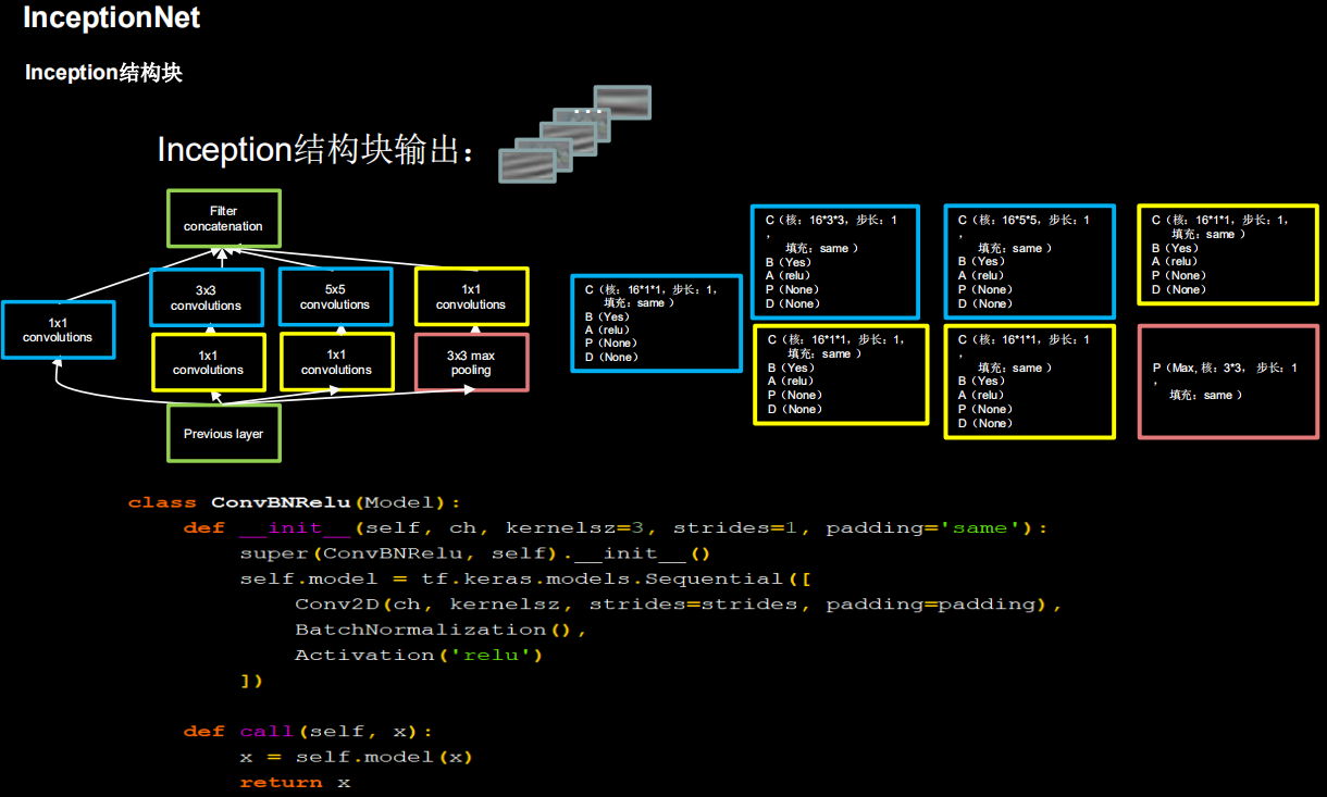
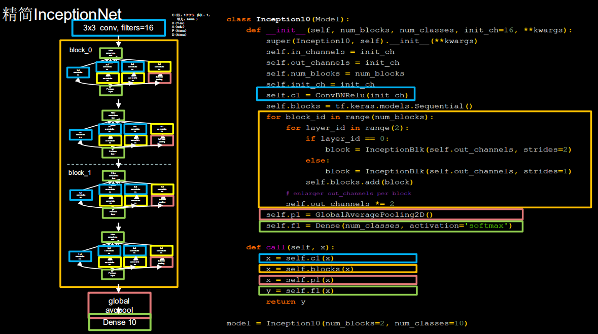
2.4.6 Inception10

import tensorflow as tf
import os
import numpy as np
from matplotlib import pyplot as plt
from tensorflow.keras.layers import Conv2D, BatchNormalization, Activation, MaxPool2D, Dropout, Flatten, Dense, \
    GlobalAveragePooling2D
from tensorflow.keras import Model

np.set_printoptions(threshold=np.inf)

cifar10 = tf.keras.datasets.cifar10
(x_train, y_train), (x_test, y_test) = cifar10.load_data()
x_train, x_test = x_train / 255.0, x_test / 255.0


class ConvBNRelu(Model):
    def __init__(self, ch, kernelsz=3, strides=1, padding='same'):
        super(ConvBNRelu, self).__init__()
        self.model = tf.keras.models.Sequential([
            Conv2D(ch, kernelsz, strides=strides, padding=padding),
            BatchNormalization(),
            Activation('relu')
        ])

    def call(self, x):
        x = self.model(x, training=False) #在training=False时，BN通过整个训练集计算均值、方差去做批归一化，training=True时，通过当前batch的均值、方差去做批归一化。推理时 training=False效果好
        return x


class InceptionBlk(Model):
    def __init__(self, ch, strides=1):
        super(InceptionBlk, self).__init__()
        self.ch = ch
        self.strides = strides
        self.c1 = ConvBNRelu(ch, kernelsz=1, strides=strides)
        self.c2_1 = ConvBNRelu(ch, kernelsz=1, strides=strides)
        self.c2_2 = ConvBNRelu(ch, kernelsz=3, strides=1)
        self.c3_1 = ConvBNRelu(ch, kernelsz=1, strides=strides)
        self.c3_2 = ConvBNRelu(ch, kernelsz=5, strides=1)
        self.p4_1 = MaxPool2D(3, strides=1, padding='same')
        self.c4_2 = ConvBNRelu(ch, kernelsz=1, strides=strides)

    def call(self, x):
        x1 = self.c1(x)
        x2_1 = self.c2_1(x)
        x2_2 = self.c2_2(x2_1)
        x3_1 = self.c3_1(x)
        x3_2 = self.c3_2(x3_1)
        x4_1 = self.p4_1(x)
        x4_2 = self.c4_2(x4_1)
        # concat along axis=channel
        x = tf.concat([x1, x2_2, x3_2, x4_2], axis=3)
        return x


class Inception10(Model):
    def __init__(self, num_blocks, num_classes, init_ch=16, **kwargs):
        super(Inception10, self).__init__(**kwargs)
        self.in_channels = init_ch
        self.out_channels = init_ch
        self.num_blocks = num_blocks
        self.init_ch = init_ch
        self.c1 = ConvBNRelu(init_ch)
        self.blocks = tf.keras.models.Sequential()
        for block_id in range(num_blocks):
            for layer_id in range(2):
                if layer_id == 0:
                    block = InceptionBlk(self.out_channels, strides=2)
                else:
                    block = InceptionBlk(self.out_channels, strides=1)
                self.blocks.add(block)
            # enlarger out_channels per block
            self.out_channels *= 2
        self.p1 = GlobalAveragePooling2D()
        self.f1 = Dense(num_classes, activation='softmax')

    def call(self, x):
        x = self.c1(x)
        x = self.blocks(x)
        x = self.p1(x)
        y = self.f1(x)
        return y


model = Inception10(num_blocks=2, num_classes=10)

model.compile(optimizer='adam',
              loss=tf.keras.losses.SparseCategoricalCrossentropy(from_logits=False),
              metrics=['sparse_categorical_accuracy'])

checkpoint_save_path = "./checkpoint/Inception10.ckpt"
if os.path.exists(checkpoint_save_path + '.index'):
    print('-------------load the model-----------------')
    model.load_weights(checkpoint_save_path)

cp_callback = tf.keras.callbacks.ModelCheckpoint(filepath=checkpoint_save_path,
                                                 save_weights_only=True,
                                                 save_best_only=True)

history = model.fit(x_train, y_train, batch_size=32, epochs=5, validation_data=(x_test, y_test), validation_freq=1,
                    callbacks=[cp_callback])
model.summary()

# print(model.trainable_variables)
file = open('./weights.txt', 'w')
for v in model.trainable_variables:
    file.write(str(v.name) + '\n')
    file.write(str(v.shape) + '\n')
    file.write(str(v.numpy()) + '\n')
file.close()

###############################################    show   ###############################################

# 显示训练集和验证集的acc和loss曲线
acc = history.history['sparse_categorical_accuracy']
val_acc = history.history['val_sparse_categorical_accuracy']
loss = history.history['loss']
val_loss = history.history['val_loss']

plt.subplot(1, 2, 1)
plt.plot(acc, label='Training Accuracy')
plt.plot(val_acc, label='Validation Accuracy')
plt.title('Training and Validation Accuracy')
plt.legend()

plt.subplot(1, 2, 2)
plt.plot(loss, label='Training Loss')
plt.plot(val_loss, label='Validation Loss')
plt.title('Training and Validation Loss')
plt.legend()
plt.show()

2.4.7 ResNet18

import tensorflow as tf
import os
import numpy as np
from matplotlib import pyplot as plt
from tensorflow.keras.layers import Conv2D, BatchNormalization, Activation, MaxPool2D, Dropout, Flatten, Dense
from tensorflow.keras import Model

np.set_printoptions(threshold=np.inf)

cifar10 = tf.keras.datasets.cifar10
(x_train, y_train), (x_test, y_test) = cifar10.load_data()
x_train, x_test = x_train / 255.0, x_test / 255.0


class ResnetBlock(Model):

    def __init__(self, filters, strides=1, residual_path=False):
        super(ResnetBlock, self).__init__()
        self.filters = filters
        self.strides = strides
        self.residual_path = residual_path

        self.c1 = Conv2D(filters, (3, 3), strides=strides, padding='same', use_bias=False)
        self.b1 = BatchNormalization()
        self.a1 = Activation('relu')

        self.c2 = Conv2D(filters, (3, 3), strides=1, padding='same', use_bias=False)
        self.b2 = BatchNormalization()

        # residual_path为True时，对输入进行下采样，即用1x1的卷积核做卷积操作，保证x能和F(x)维度相同，顺利相加
        if residual_path:
            self.down_c1 = Conv2D(filters, (1, 1), strides=strides, padding='same', use_bias=False)
            self.down_b1 = BatchNormalization()
        
        self.a2 = Activation('relu')

    def call(self, inputs):
        residual = inputs  # residual等于输入值本身，即residual=x
        # 将输入通过卷积、BN层、激活层，计算F(x)
        x = self.c1(inputs)
        x = self.b1(x)
        x = self.a1(x)

        x = self.c2(x)
        y = self.b2(x)

        if self.residual_path:
            residual = self.down_c1(inputs)
            residual = self.down_b1(residual)

        out = self.a2(y + residual)  # 最后输出的是两部分的和，即F(x)+x或F(x)+Wx,再过激活函数
        return out


class ResNet18(Model):

    def __init__(self, block_list, initial_filters=64):  # block_list表示每个block有几个卷积层
        super(ResNet18, self).__init__()
        self.num_blocks = len(block_list)  # 共有几个block
        self.block_list = block_list
        self.out_filters = initial_filters
        self.c1 = Conv2D(self.out_filters, (3, 3), strides=1, padding='same', use_bias=False)
        self.b1 = BatchNormalization()
        self.a1 = Activation('relu')
        self.blocks = tf.keras.models.Sequential()
        # 构建ResNet网络结构
        for block_id in range(len(block_list)):  # 第几个resnet block
            for layer_id in range(block_list[block_id]):  # 第几个卷积层

                if block_id != 0 and layer_id == 0:  # 对除第一个block以外的每个block的输入进行下采样
                    block = ResnetBlock(self.out_filters, strides=2, residual_path=True)
                else:
                    block = ResnetBlock(self.out_filters, residual_path=False)
                self.blocks.add(block)  # 将构建好的block加入resnet
            self.out_filters *= 2  # 下一个block的卷积核数是上一个block的2倍
        self.p1 = tf.keras.layers.GlobalAveragePooling2D()
        self.f1 = tf.keras.layers.Dense(10, activation='softmax', kernel_regularizer=tf.keras.regularizers.l2())

    def call(self, inputs):
        x = self.c1(inputs)
        x = self.b1(x)
        x = self.a1(x)
        x = self.blocks(x)
        x = self.p1(x)
        y = self.f1(x)
        return y


model = ResNet18([2, 2, 2, 2])

model.compile(optimizer='adam',
              loss=tf.keras.losses.SparseCategoricalCrossentropy(from_logits=False),
              metrics=['sparse_categorical_accuracy'])

checkpoint_save_path = "./checkpoint/ResNet18.ckpt"
if os.path.exists(checkpoint_save_path + '.index'):
    print('-------------load the model-----------------')
    model.load_weights(checkpoint_save_path)

cp_callback = tf.keras.callbacks.ModelCheckpoint(filepath=checkpoint_save_path,
                                                 save_weights_only=True,
                                                 save_best_only=True)

history = model.fit(x_train, y_train, batch_size=32, epochs=5, validation_data=(x_test, y_test), validation_freq=1,
                    callbacks=[cp_callback])
model.summary()

# print(model.trainable_variables)
file = open('./weights.txt', 'w')
for v in model.trainable_variables:
    file.write(str(v.name) + '\n')
    file.write(str(v.shape) + '\n')
    file.write(str(v.numpy()) + '\n')
file.close()

###############################################    show   ###############################################

# 显示训练集和验证集的acc和loss曲线
acc = history.history['sparse_categorical_accuracy']
val_acc = history.history['val_sparse_categorical_accuracy']
loss = history.history['loss']
val_loss = history.history['val_loss']

plt.subplot(1, 2, 1)
plt.plot(acc, label='Training Accuracy')
plt.plot(val_acc, label='Validation Accuracy')
plt.title('Training and Validation Accuracy')
plt.legend()

plt.subplot(1, 2, 2)
plt.plot(loss, label='Training Loss')
plt.plot(val_loss, label='Validation Loss')
plt.title('Training and Validation Loss')
plt.legend()
plt.show()

3 机器学习常见知识点代码实现

在不断完善中…

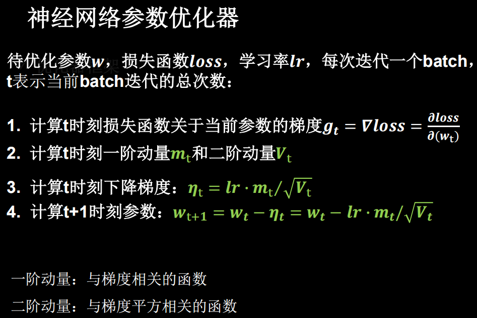
3.1 常用的优化器的代码实现

▲ 优化器的数学原理

3.1.1 SGD

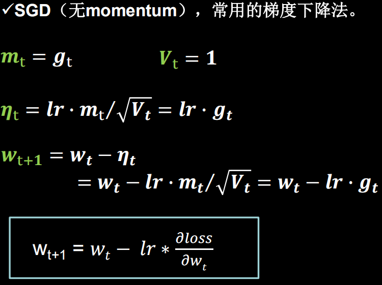
for epoch in range(epoch):  # 数据集级别的循环，每个epoch循环一次数据集
    for step, (x_train, y_train) in enumerate(train_db):  # batch级别的循环 ，每个step循环一个batch
        with tf.GradientTape() as tape:  # with结构记录梯度信息
            y = tf.matmul(x_train, w1) + b1  # 神经网络乘加运算
            y = tf.nn.softmax(y)  # 使输出y符合概率分布（此操作后与独热码同量级，可相减求loss）
            y_ = tf.one_hot(y_train, depth=3)  # 将标签值转换为独热码格式，方便计算loss和accuracy
            loss = tf.reduce_mean(tf.square(y_ - y))  # 采用均方误差损失函数mse = mean(sum(y-out)^2)
            loss_all += loss.numpy()  # 将Tensor变量转换为ndarray变量，将每个step计算出的loss累加，为后续求loss平均值提供数据，这样计算的loss更准确
        # 计算loss对各个参数的梯度
        grads = tape.gradient(loss, [w1, b1])

        # 实现梯度更新 w1 = w1 - lr * w1_grad    b = b - lr * b_grad
        w1.assign_sub(lr * grads[0])  # 参数w1自更新
        b1.assign_sub(lr * grads[1])  # 参数b自更新

3.1.2 SGDM

	##########################################################################
m_w, m_b = 0, 0
beta = 0.9
##########################################################################

# 训练部分
now_time = time.time()  ##2##
for epoch in range(epoch):  # 数据集级别的循环，每个epoch循环一次数据集
    for step, (x_train, y_train) in enumerate(train_db):  # batch级别的循环 ，每个step循环一个batch
        with tf.GradientTape() as tape:  # with结构记录梯度信息
            y = tf.matmul(x_train, w1) + b1  # 神经网络乘加运算
            y = tf.nn.softmax(y)  # 使输出y符合概率分布（此操作后与独热码同量级，可相减求loss）
            y_ = tf.one_hot(y_train, depth=3)  # 将标签值转换为独热码格式，方便计算loss和accuracy
            loss = tf.reduce_mean(tf.square(y_ - y))  # 采用均方误差损失函数mse = mean(sum(y-out)^2)
            loss_all += loss.numpy()  # 将每个step计算出的loss累加，为后续求loss平均值提供数据，这样计算的loss更准确
        # 计算loss对各个参数的梯度
        grads = tape.gradient(loss, [w1, b1])

        ##########################################################################
        # sgd-momentun  
        m_w = beta * m_w + (1 - beta) * grads[0]
        m_b = beta * m_b + (1 - beta) * grads[1]
        w1.assign_sub(lr * m_w)
        b1.assign_sub(lr * m_b)
    ##########################################################################

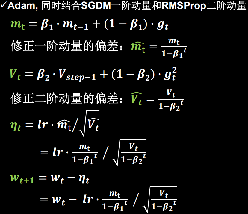
3.1.3 Adam

##########################################################################
m_w, m_b = 0, 0
v_w, v_b = 0, 0
beta1, beta2 = 0.9, 0.999
delta_w, delta_b = 0, 0
global_step = 0
##########################################################################

# 训练部分
now_time = time.time()  ##2##
for epoch in range(epoch):  # 数据集级别的循环，每个epoch循环一次数据集
    for step, (x_train, y_train) in enumerate(train_db):  # batch级别的循环 ，每个step循环一个batch
 ##########################################################################       
        global_step += 1
 ##########################################################################       
        with tf.GradientTape() as tape:  # with结构记录梯度信息
            y = tf.matmul(x_train, w1) + b1  # 神经网络乘加运算
            y = tf.nn.softmax(y)  # 使输出y符合概率分布（此操作后与独热码同量级，可相减求loss）
            y_ = tf.one_hot(y_train, depth=3)  # 将标签值转换为独热码格式，方便计算loss和accuracy
            loss = tf.reduce_mean(tf.square(y_ - y))  # 采用均方误差损失函数mse = mean(sum(y-out)^2)
            loss_all += loss.numpy()  # 将每个step计算出的loss累加，为后续求loss平均值提供数据，这样计算的loss更准确
        # 计算loss对各个参数的梯度
        grads = tape.gradient(loss, [w1, b1])

##########################################################################
 # adam
        m_w = beta1 * m_w + (1 - beta1) * grads[0]
        m_b = beta1 * m_b + (1 - beta1) * grads[1]
        v_w = beta2 * v_w + (1 - beta2) * tf.square(grads[0])
        v_b = beta2 * v_b + (1 - beta2) * tf.square(grads[1])

        m_w_correction = m_w / (1 - tf.pow(beta1, int(global_step)))
        m_b_correction = m_b / (1 - tf.pow(beta1, int(global_step)))
        v_w_correction = v_w / (1 - tf.pow(beta2, int(global_step)))
        v_b_correction = v_b / (1 - tf.pow(beta2, int(global_step)))

        w1.assign_sub(lr * m_w_correction / tf.sqrt(v_w_correction))
        b1.assign_sub(lr * m_b_correction / tf.sqrt(v_b_correction))
##########################################################################

3.1.4 Adagrad

##########################################################################
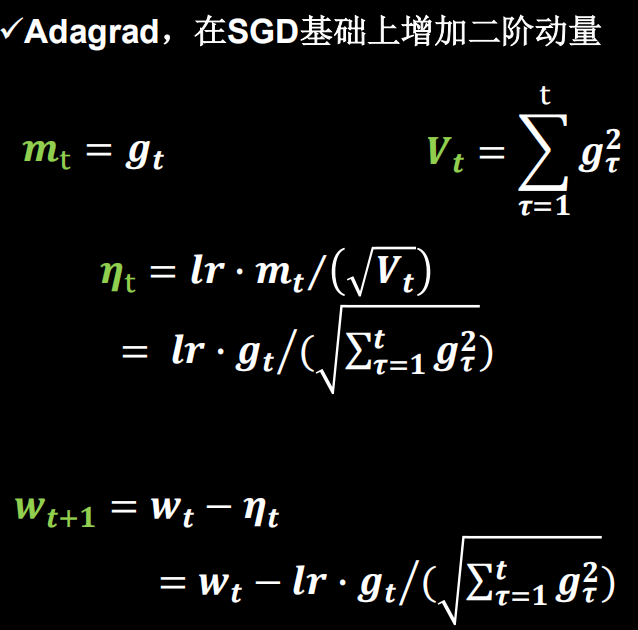
v_w, v_b = 0, 0
##########################################################################

# 训练部分
now_time = time.time()  ##2##
for epoch in range(epoch):  # 数据集级别的循环，每个epoch循环一次数据集
    for step, (x_train, y_train) in enumerate(train_db):  # batch级别的循环 ，每个step循环一个batch
        with tf.GradientTape() as tape:  # with结构记录梯度信息
            y = tf.matmul(x_train, w1) + b1  # 神经网络乘加运算
            y = tf.nn.softmax(y)  # 使输出y符合概率分布（此操作后与独热码同量级，可相减求loss）
            y_ = tf.one_hot(y_train, depth=3)  # 将标签值转换为独热码格式，方便计算loss和accuracy
            loss = tf.reduce_mean(tf.square(y_ - y))  # 采用均方误差损失函数mse = mean(sum(y-out)^2)
            loss_all += loss.numpy()  # 将每个step计算出的loss累加，为后续求loss平均值提供数据，这样计算的loss更准确
        # 计算loss对各个参数的梯度
        grads = tape.gradient(loss, [w1, b1])

        ##########################################################################
        # adagrad
        v_w += tf.square(grads[0])
        v_b += tf.square(grads[1])
        w1.assign_sub(lr * grads[0] / tf.sqrt(v_w))
        b1.assign_sub(lr * grads[1] / tf.sqrt(v_b))
    ##########################################################################

3.1.5 Rmsprop

##########################################################################
v_w, v_b = 0, 0
beta = 0.9
##########################################################################

# 训练部分
now_time = time.time()  ##2##
for epoch in range(epoch):  # 数据集级别的循环，每个epoch循环一次数据集
    for step, (x_train, y_train) in enumerate(train_db):  # batch级别的循环 ，每个step循环一个batch
        with tf.GradientTape() as tape:  # with结构记录梯度信息
            y = tf.matmul(x_train, w1) + b1  # 神经网络乘加运算
            y = tf.nn.softmax(y)  # 使输出y符合概率分布（此操作后与独热码同量级，可相减求loss）
            y_ = tf.one_hot(y_train, depth=3)  # 将标签值转换为独热码格式，方便计算loss和accuracy
            loss = tf.reduce_mean(tf.square(y_ - y))  # 采用均方误差损失函数mse = mean(sum(y-out)^2)
            loss_all += loss.numpy()  # 将每个step计算出的loss累加，为后续求loss平均值提供数据，这样计算的loss更准确
        # 计算loss对各个参数的梯度
        grads = tape.gradient(loss, [w1, b1])

        ##########################################################################
        # rmsprop
        v_w = beta * v_w + (1 - beta) * tf.square(grads[0])
        v_b = beta * v_b + (1 - beta) * tf.square(grads[1])
        w1.assign_sub(lr * grads[0] / tf.sqrt(v_w))
        b1.assign_sub(lr * grads[1] / tf.sqrt(v_b))
    ##########################################################################