内容来自:https://pytorch.org/tutorials/beginner/transfer_learning_tutorial.html
在这篇教程中,我们将学会如何使用迁移学习来训练自己的网络。在cs231n notes上有更多关于迁移学习的介绍。
概括如下:
在实际中,几乎没有人会从头去训练整个卷积神经网络(基本没有进行初始化的),因为通常很难拥有充足的数据支持训练工作。相反的,我们通常在大型数据集上(例如ImageNet,包含了120万张、1000类图片)进行预训练卷积网络,然后利用该卷积网络为目标任务做初始化,或固定特征的提取器。
迁移学习两个主要的应用场景:
- 卷积网络的微调 :我们先在imagenet数据集上预训练,用预训练的结果初始化网络,剩下的训练工作照常进行。
- 固定特征提取器:我们会冻结预训练后,最后全连接层之外的网络权重。然后用一组随机权重生成新的全连接层,对该层进行训练。
# License: BSD
# Author: Sasank Chilamkurthy

from __future__ import print_function, division

import torch
import torch.nn as nn
import torch.optim as optim
from torch.optim import lr_scheduler
import numpy as np
import torchvision
from torchvision import datasets, models, transforms
import matplotlib.pyplot as plt
import time
import os
import copy

plt.ion()   # interactive mode
载入数据 Load Data
我们使用torchvision和torch.utils.data包来载入数据。
今天的案例是训练一个模型,对蚂蚁和蜜蜂进行分类。对于蚂蚁、蜜蜂我们各有120张训练图片;每类有75张验证图片。通常,如果从头开始训练,只能从很小的数据集上提取特征。现在我们学习了迁移学习,就能够合理的进行特征提取。
数据集下载入口:点击这里
# Data augmentation and normalization for training
# Just normalization for validation
data_transforms = {
    'train': transforms.Compose([
        transforms.RandomResizedCrop(224),
        transforms.RandomHorizontalFlip(),
        transforms.ToTensor(),
        transforms.Normalize([0.485, 0.456, 0.406], [0.229, 0.224, 0.225])
    ]),
    'val': transforms.Compose([
        transforms.Resize(256),
        transforms.CenterCrop(224),
        transforms.ToTensor(),
        transforms.Normalize([0.485, 0.456, 0.406], [0.229, 0.224, 0.225])
    ]),
}

data_dir = 'data/hymenoptera_data'
image_datasets = {x: datasets.ImageFolder(os.path.join(data_dir, x),
                                          data_transforms[x])
                  for x in ['train', 'val']}
dataloaders = {x: torch.utils.data.DataLoader(image_datasets[x], batch_size=4,
                                             shuffle=True, num_workers=4)
              for x in ['train', 'val']}
dataset_sizes = {x: len(image_datasets[x]) for x in ['train', 'val']}
class_names = image_datasets['train'].classes

device = torch.device("cuda:0" if torch.cuda.is_available() else "cpu")
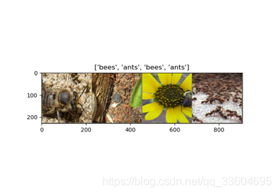
图像可视化 Visualize a few images
下面我们将少部分图片展示出来,以此来理解数据增强。
def imshow(inp, title=None):
    """Imshow for Tensor."""
    inp = inp.numpy().transpose((1, 2, 0))
    mean = np.array([0.485, 0.456, 0.406])
    std = np.array([0.229, 0.224, 0.225])
    inp = std * inp + mean
    inp = np.clip(inp, 0, 1)
    plt.imshow(inp)
    if title is not None:
        plt.title(title)
    plt.pause(0.001)  # pause a bit so that plots are updated


# Get a batch of training data
inputs, classes = next(iter(dataloaders['train']))

# Make a grid from batch
out = torchvision.utils.make_grid(inputs)

imshow(out, title=[class_names[x] for x in classes])
训练模型 Training the model
现在,我们写一个通用的函数来训练模型,并展示以下内容:
- 设计学习率
- 保存最佳模型
下面的示例中,参数scheduler是一个专门用来设置学习率的对象,继承自torch.optim.lr_scheduler。
def train_model(model, criterion, optimizer, scheduler, num_epochs=25):
    since = time.time()

    best_model_wts = copy.deepcopy(model.state_dict())
    best_acc = 0.0

    for epoch in range(num_epochs):
        print('Epoch {}/{}'.format(epoch, num_epochs - 1))
        print('-' * 10)

        # Each epoch has a training and validation phase
        for phase in ['train', 'val']:
            if phase == 'train':
                scheduler.step()
                model.train()  # Set model to training mode
            else:
                model.eval()   # Set model to evaluate mode

            running_loss = 0.0
            running_corrects = 0

            # Iterate over data.
            for inputs, labels in dataloaders[phase]:
                inputs = inputs.to(device)
                labels = labels.to(device)

                # zero the parameter gradients
                optimizer.zero_grad()

                # forward
                # track history if only in train
                with torch.set_grad_enabled(phase == 'train'):
                    outputs = model(inputs)
                    _, preds = torch.max(outputs, 1)
                    loss = criterion(outputs, labels)

                    # backward + optimize only if in training phase
                    if phase == 'train':
                        loss.backward()
                        optimizer.step()

                # statistics
                running_loss += loss.item() * inputs.size(0)
                running_corrects += torch.sum(preds == labels.data)

            epoch_loss = running_loss / dataset_sizes[phase]
            epoch_acc = running_corrects.double() / dataset_sizes[phase]

            print('{} Loss: {:.4f} Acc: {:.4f}'.format(
                phase, epoch_loss, epoch_acc))

            # deep copy the model
            if phase == 'val' and epoch_acc > best_acc:
                best_acc = epoch_acc
                best_model_wts = copy.deepcopy(model.state_dict())

        print()

    time_elapsed = time.time() - since
    print('Training complete in {:.0f}m {:.0f}s'.format(
        time_elapsed // 60, time_elapsed % 60))
    print('Best val Acc: {:4f}'.format(best_acc))

    # load best model weights
    model.load_state_dict(best_model_wts)
    return model
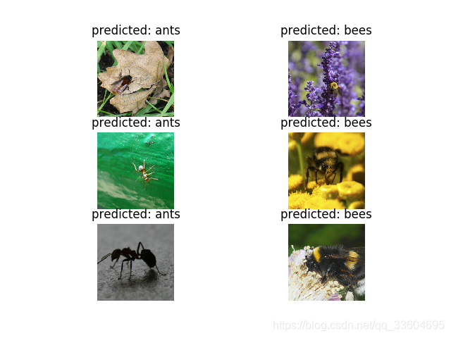
显示模型预测结果 Visualizing the model predictions
下面展示出一些图片的预测结果:
def visualize_model(model, num_images=6):
    was_training = model.training
    model.eval()
    images_so_far = 0
    fig = plt.figure()

    with torch.no_grad():
        for i, (inputs, labels) in enumerate(dataloaders['val']):
            inputs = inputs.to(device)
            labels = labels.to(device)

            outputs = model(inputs)
            _, preds = torch.max(outputs, 1)

            for j in range(inputs.size()[0]):
                images_so_far += 1
                ax = plt.subplot(num_images//2, 2, images_so_far)
                ax.axis('off')
                ax.set_title('predicted: {}'.format(class_names[preds[j]]))
                imshow(inputs.cpu().data[j])

                if images_so_far == num_images:
                    model.train(mode=was_training)
                    return
        model.train(mode=was_training)
微调卷积网络 Finetuning the convnet
加载预测里模型,并重置最后的全连接层。
model_ft = models.resnet18(pretrained=True)
num_ftrs = model_ft.fc.in_features
model_ft.fc = nn.Linear(num_ftrs, 2)

model_ft = model_ft.to(device)

criterion = nn.CrossEntropyLoss()

# Observe that all parameters are being optimized
optimizer_ft = optim.SGD(model_ft.parameters(), lr=0.001, momentum=0.9)

# Decay LR by a factor of 0.1 every 7 epochs
exp_lr_scheduler = lr_scheduler.StepLR(optimizer_ft, step_size=7, gamma=0.1)
训练和评估(一) Train and evaluate
在CPU上训练需要15-25min,GPU上花费不到1min。
model_ft = train_model(model_ft, criterion, optimizer_ft, exp_lr_scheduler,
                       num_epochs=25)
输出如下:
Epoch 0/24
----------
train Loss: 0.7032 Acc: 0.6025
val Loss: 0.1698 Acc: 0.9412

Epoch 1/24
----------
train Loss: 0.6411 Acc: 0.7787
val Loss: 0.1981 Acc: 0.9281

Epoch 2/24
----------
train Loss: 0.3053 Acc: 0.8648
val Loss: 0.2216 Acc: 0.9281

Epoch 3/24
----------
train Loss: 0.4394 Acc: 0.8238
val Loss: 0.2952 Acc: 0.8889

Epoch 4/24
----------
train Loss: 0.6016 Acc: 0.7828
val Loss: 0.6002 Acc: 0.8366

Epoch 5/24
----------
train Loss: 0.6057 Acc: 0.8279
val Loss: 0.4083 Acc: 0.8693

Epoch 6/24
----------
train Loss: 0.3448 Acc: 0.8648
val Loss: 0.3406 Acc: 0.8889

Epoch 7/24
----------
train Loss: 0.4521 Acc: 0.8361
val Loss: 0.3086 Acc: 0.8954

Epoch 8/24
----------
train Loss: 0.3378 Acc: 0.8566
val Loss: 0.3197 Acc: 0.9020

Epoch 9/24
----------
train Loss: 0.3723 Acc: 0.8361
val Loss: 0.3028 Acc: 0.9020

Epoch 10/24
----------
train Loss: 0.3645 Acc: 0.8279
val Loss: 0.2656 Acc: 0.9281

Epoch 11/24
----------
train Loss: 0.2905 Acc: 0.8730
val Loss: 0.2649 Acc: 0.9216

Epoch 12/24
----------
train Loss: 0.2931 Acc: 0.8730
val Loss: 0.2416 Acc: 0.9150

Epoch 13/24
----------
train Loss: 0.2846 Acc: 0.8770
val Loss: 0.2413 Acc: 0.9216

Epoch 14/24
----------
train Loss: 0.2775 Acc: 0.8648
val Loss: 0.2478 Acc: 0.9281

Epoch 15/24
----------
train Loss: 0.2860 Acc: 0.8975
val Loss: 0.2491 Acc: 0.9216

Epoch 16/24
----------
train Loss: 0.2707 Acc: 0.8852
val Loss: 0.2471 Acc: 0.9150

Epoch 17/24
----------
train Loss: 0.3009 Acc: 0.8730
val Loss: 0.2385 Acc: 0.9216

Epoch 18/24
----------
train Loss: 0.2415 Acc: 0.8934
val Loss: 0.2465 Acc: 0.9216

Epoch 19/24
----------
train Loss: 0.2520 Acc: 0.9057
val Loss: 0.2898 Acc: 0.8954

Epoch 20/24
----------
train Loss: 0.3212 Acc: 0.8525
val Loss: 0.2545 Acc: 0.9216

Epoch 21/24
----------
train Loss: 0.3919 Acc: 0.8279
val Loss: 0.2310 Acc: 0.9216

Epoch 22/24
----------
train Loss: 0.3334 Acc: 0.8484
val Loss: 0.2542 Acc: 0.9085

Epoch 23/24
----------
train Loss: 0.2734 Acc: 0.8934
val Loss: 0.2614 Acc: 0.9150

Epoch 24/24
----------
train Loss: 0.2812 Acc: 0.8730
val Loss: 0.2647 Acc: 0.9150

Training complete in 1m 7s
Best val Acc: 0.941176
visualize_model(model_ft)
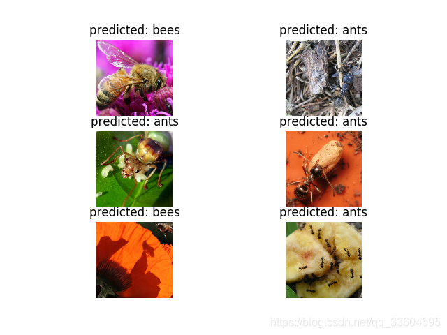
冻结卷积网络作为固定特征提取器 ConvNet as fixed feature extractor
在这步,我们需要冻结最后全连接层以外的网络。设置requires_grad == False来冻结权重参数,这样在反向传播backward()时,不再计算相应的梯度。
点击这里获取更多的相关介绍。
model_conv = torchvision.models.resnet18(pretrained=True)
for param in model_conv.parameters():
    param.requires_grad = False

# Parameters of newly constructed modules have requires_grad=True by default
num_ftrs = model_conv.fc.in_features
model_conv.fc = nn.Linear(num_ftrs, 2)

model_conv = model_conv.to(device)

criterion = nn.CrossEntropyLoss()

# Observe that only parameters of final layer are being optimized as
# opposed to before.
optimizer_conv = optim.SGD(model_conv.fc.parameters(), lr=0.001, momentum=0.9)

# Decay LR by a factor of 0.1 every 7 epochs
exp_lr_scheduler = lr_scheduler.StepLR(optimizer_conv, step_size=7, gamma=0.1)
训练和评估(二) Train and evaluate
在CPU上训练的时间大约是之前的一半,这是由于大多数中间层的梯度都不用再计算,但是向前传播过程仍需要计算。
model_conv = train_model(model_conv, criterion, optimizer_conv,
                         exp_lr_scheduler, num_epochs=25)
输出为:
Epoch 0/24
----------
train Loss: 0.6400 Acc: 0.6434
val Loss: 0.2539 Acc: 0.9085

Epoch 1/24
----------
train Loss: 0.6115 Acc: 0.7541
val Loss: 0.2492 Acc: 0.9216

Epoch 2/24
----------
train Loss: 0.5561 Acc: 0.7828
val Loss: 0.2039 Acc: 0.9412

Epoch 3/24
----------
train Loss: 0.5970 Acc: 0.7541
val Loss: 0.1834 Acc: 0.9542

Epoch 4/24
----------
train Loss: 0.3666 Acc: 0.8320
val Loss: 0.2399 Acc: 0.9281

Epoch 5/24
----------
train Loss: 0.4242 Acc: 0.8279
val Loss: 0.2105 Acc: 0.9412

Epoch 6/24
----------
train Loss: 0.4163 Acc: 0.7951
val Loss: 0.1988 Acc: 0.9477

Epoch 7/24
----------
train Loss: 0.3409 Acc: 0.8566
val Loss: 0.2007 Acc: 0.9477

Epoch 8/24
----------
train Loss: 0.3756 Acc: 0.8156
val Loss: 0.2218 Acc: 0.9346

Epoch 9/24
----------
train Loss: 0.3495 Acc: 0.8320
val Loss: 0.1902 Acc: 0.9477

Epoch 10/24
----------
train Loss: 0.3385 Acc: 0.8279
val Loss: 0.2184 Acc: 0.9412

Epoch 11/24
----------
train Loss: 0.2559 Acc: 0.8811
val Loss: 0.2067 Acc: 0.9412

Epoch 12/24
----------
train Loss: 0.3974 Acc: 0.7992
val Loss: 0.2046 Acc: 0.9477

Epoch 13/24
----------
train Loss: 0.3274 Acc: 0.8525
val Loss: 0.2272 Acc: 0.9346

Epoch 14/24
----------
train Loss: 0.3668 Acc: 0.8525
val Loss: 0.2309 Acc: 0.9150

Epoch 15/24
----------
train Loss: 0.3485 Acc: 0.8484
val Loss: 0.1984 Acc: 0.9412

Epoch 16/24
----------
train Loss: 0.3573 Acc: 0.8115
val Loss: 0.2180 Acc: 0.9346

Epoch 17/24
----------
train Loss: 0.2899 Acc: 0.8770
val Loss: 0.1984 Acc: 0.9412

Epoch 18/24
----------
train Loss: 0.3893 Acc: 0.8402
val Loss: 0.2189 Acc: 0.9477

Epoch 19/24
----------
train Loss: 0.2820 Acc: 0.8934
val Loss: 0.2297 Acc: 0.9281

Epoch 20/24
----------
train Loss: 0.2569 Acc: 0.8730
val Loss: 0.2088 Acc: 0.9477

Epoch 21/24
----------
train Loss: 0.3154 Acc: 0.8689
val Loss: 0.2243 Acc: 0.9216

Epoch 22/24
----------
train Loss: 0.2780 Acc: 0.8648
val Loss: 0.1942 Acc: 0.9346

Epoch 23/24
----------
train Loss: 0.2988 Acc: 0.8607
val Loss: 0.2151 Acc: 0.9412

Epoch 24/24
----------
train Loss: 0.3519 Acc: 0.8484
val Loss: 0.2045 Acc: 0.9412

Training complete in 0m 35s
Best val Acc: 0.954248
visualize_model(model_conv)

plt.ioff()
plt.show()