python使用numpy模块的介绍，基本操作，处理数据，包括生成数组，正态分布，均匀数组，数值改变，索引切片，形状修改，类型修改,数组去重，值运算，数组运算，合并分割，IO操作（读取）

初学阶段，可以认为numpy的某些方法也可以运用到pandas模块中，例如np.where（）三元运算、unique去重方法、shape方法

1 Numpy介绍

Numpy（Numerical Python）是一个开源的Python科学计算库，用于快速处理任意维度的数组。
Numpy支持常见的数组和矩阵操作。对于同样的数值计算任务，使用Numpy比直接使用Python要简洁的多。
Numpy使用ndarray对象来处理多维数组，该对象是一个快速而灵活的大数据容器。

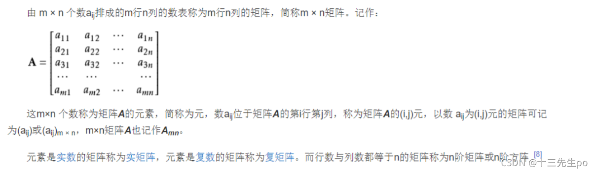
2 ndarray介绍

NumPy提供了一个N维数组类型ndarray，它描述了相同类型的“items”的集合。

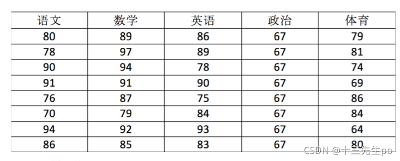
用ndarray进行存储：

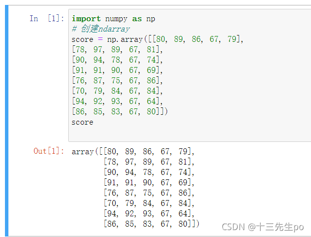
简单创建一个array类型数据

import numpy as np
# 创建ndarray
score = np.array([[80, 89, 86, 67, 79],
[78, 97, 89, 67, 81],
[90, 94, 78, 67, 74],
[91, 91, 90, 67, 69],
[76, 87, 75, 67, 86],
[70, 79, 84, 67, 84],
[94, 92, 93, 67, 64],
[86, 85, 83, 67, 80]])
score

ndarray与Python原生list运算效率对比以及举例代码

在这里我们通过一段带运行来体会到ndarray的好处

import random 
import time 
import numpy as np

a=[]
for i in range(100000000):
    a.append(random.random())
    
t1 = time.time()
sum1 = sum(a)
t2 = time.time()

b = np.array(a)
t4 = time.time()
sum3 = np.sum(b)
t5 = time.time()
#t2-t1为使用python自带的求和函数消耗的时间，t5-t4为使用numpy求和消耗的时间，结果为：
print(t2-t1,t5-t4)

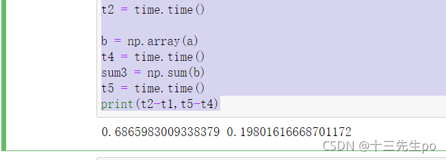
从中我们看到ndarray的计算速度要快很多，节约了时间。

• 机器学习的最大特点就是大量的数据运算，那么如果没有一个快速的解决方案，那可能现在python也在机器学习领域达不到好的效果。
  
  Numpy专门针对ndarray的操作和运算进行了设计，所以数组的存储效率和输入输出性能远优于Python中的嵌套列表，数组越大，Numpy的优势就越明显。

3 N维数组-ndarray

ndarray的属性

数组属性反映了数组本身固有的信息。

属性名字	属性解释
ndarray.shape	数组维度的元组
ndarray.ndim	数组维数
ndarray.size	数组中的元素数量
ndarray.itemsize	一个数组元素的长度（字节）
ndarray.dtype	数组元素的类型

ndarray的形状(ndarray.shape)

numpy的array结构和pandas的dataframe结构一样都可以调用查看shape属性

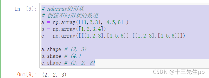
# ndarray的形状
# 创建不同形状的数组
a = np.array([[1,2,3],[4,5,6]])
b = np.array([1,2,3,4])
c = np.array([[[1,2,3],[4,5,6]],[[1,2,3],[4,5,6]]])

a.shape # (2, 3) # 二维数组
b.shape # (4,) # 一维数组
c.shape # (2, 2, 3)  # 三维数组

ndarray的类型(ndarray.dtype)

• 注意：若不指定，整数默认int64，小数默认float64

名称	描述	简写
np.bool	用一个字节存储的布尔类型（True或False）	‘b’
np.int8	一个字节大小，-128 至 127	‘i’
np.int16	整数，-32768 至 32767	‘i2’
np.int32	整数，-2 31 至 2 32 -1	‘i4’
np.int64	整数，-2 63 至 2 63 - 1	‘i8’
np.uint8	无符号整数，0 至 255	‘u’
np.uint16	无符号整数，0 至 65535	‘u2’
np.uint32	无符号整数，0 至 2 ** 32 - 1	‘u4’
np.uint64	无符号整数，0 至 2 ** 64 - 1	‘u8’
np.float16	半精度浮点数：16位，正负号1位，指数5位，精度10位	‘f2’
np.float32	单精度浮点数：32位，正负号1位，指数8位，精度23位	‘f4’
np.float64	双精度浮点数：64位，正负号1位，指数11位，精度52位	‘f8’
np.complex64	复数，分别用两个32位浮点数表示实部和虚部	‘c8’
np.complex128	复数，分别用两个64位浮点数表示实部和虚部	‘c16’
np.object_	python对象	‘O’
np.string_	字符串	‘S’
np.unicode_	unicode类型	‘U’

举例代码

#  ndarray的类型
a = np.array([[1, 2, 3],[4, 5, 6]], dtype=np.float32)
a.dtype  # dtype('float32')

arr = np.array(['python', 'tensorflow', 'scikit-learn', 'numpy'], dtype =
np.string_)
arr.dtype # dtype('S12')

3.1基本操作

3.1.1生成数组的方法

1 生成0和1的数组

• empty(shape[, dtype, order]) empty_like(a[, dtype, order, subok])
• eye(N[, M, k, dtype, order])
• identity(n[, dtype])
• ones(shape[, dtype, order])
• ones_like(a[, dtype, order, subok])
• zeros(shape[, dtype, order]) # 常用
• zeros_like(a[, dtype, order, subok])
• full(shape, fill_value[, dtype, order])
• full_like(a, fill_value[, dtype, order, subok])

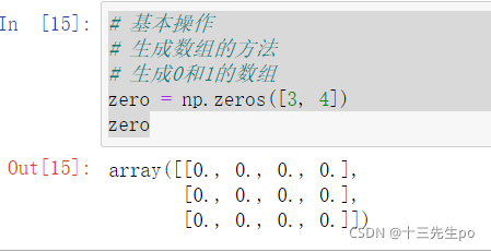
# 基本操作
# 生成数组的方法
# 生成0和1的数组
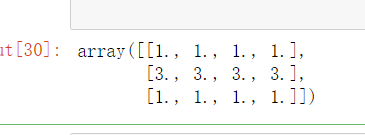
zero = np.zeros([3, 4])
zero

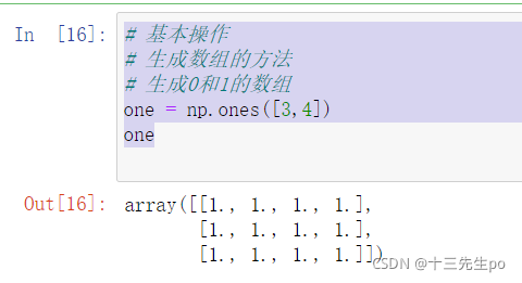
# 基本操作
# 生成数组的方法
# 生成0和1的数组
one = np.ones([3,4])
one

2 从现有数组生成

• array(object[, dtype, copy, order, subok, ndmin])
• asarray(a[, dtype, order])
• asanyarray(a[, dtype, order])
• ascontiguousarray(a[, dtype])
• asmatrix(data[, dtype])
• copy(a[, order])

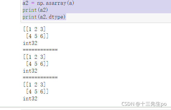
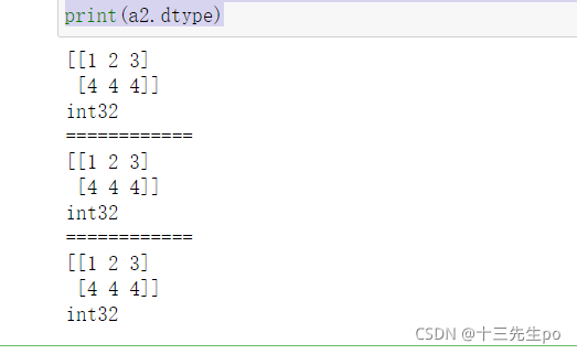
# 基本操作
# 生成数组的方法
# 2 从现有数组生成
a = np.array([[1,2,3],[4,5,6]])
print(a)
print(a.dtype)
print('============')
# 从现有的数组当中创建
a1 = np.array(a)
print(a1)
print(a1.dtype)
print('============')
# 相当于索引的形式，并没有真正的创建一个新的
a2 = np.asarray(a)
print(a2)
print(a2.dtype)

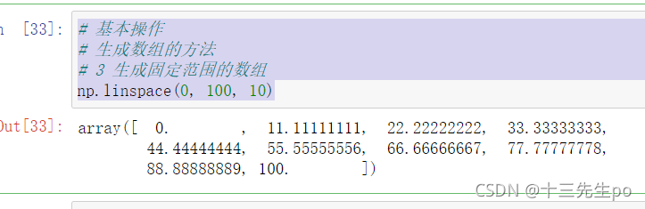
3 生成固定范围的数组

• np.linspace (start, stop, num, endpoint, retstep, dtype)
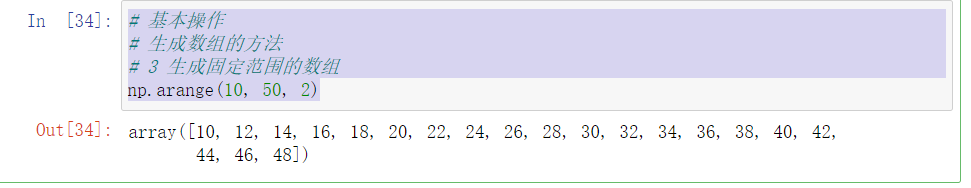
  生成等间隔的序列
• numpy.arange(start,stop, step, dtype)
• numpy.logspace(start,stop, num, endpoint, base, dtype)

start 序列的起始值
stop 序列的终止值，
如果endpoint为true，该值包含于序列中
num 要生成的等间隔样例数量，默认为50
endpoint 序列中是否包含stop值，默认为ture
retstep 如果为true，返回样例，
以及连续数字之间的步长
dtype 输出ndarray的数据类型

# 基本操作
# 生成数组的方法
# 3 生成固定范围的数组
np.linspace(0, 100, 10)

# 基本操作
# 生成数组的方法
# 3 生成固定范围的数组
np.arange(10, 50, 2)

4 生成随机数组

• np.random模块
  • 均匀分布
    • np.random.rand(d0, d1, …, dn)
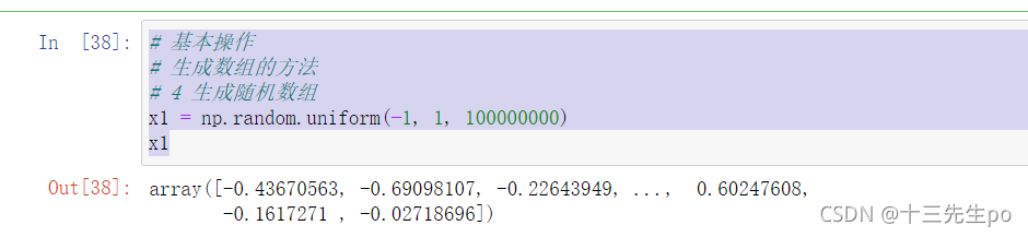
      返回[0.0，1.0)内的一组均匀分布的数。
    • np.random.uniform(low=0.0, high=1.0, size=None)
      功能：从一个均匀分布[low,high)中随机采样，注意定义域是左闭右开，即包含low，不
      包含high.
      参数介绍:
      low: 采样下界，float类型，默认值为0；
      high: 采样上界，float类型，默认值为1；
      size: 输出样本数目，为int或元组(tuple)类型，例如，size=(m,n,k), 则输出mnk个样
      本，缺省时输出1个值。
      返回值：ndarray类型，其形状和参数size中描述一致。
    • np.random.randint(low, high=None, size=None, dtype=‘l’)
      从一个均匀分布中随机采样，生成一个整数或N维整数数组，取数范围：若high不为
      None时，取[low,high)之间随机整数，否则取值[0,low)之间随机整数。

# 基本操作
# 生成数组的方法
# 4 生成随机数组
x1 = np.random.uniform(-1, 1, 100000000)
x1

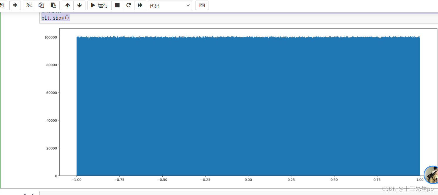
画图看分布状况：

# 基本操作
# 生成数组的方法
# 4 生成随机数组
# 画图看分布状况：
import matplotlib.pyplot as plt

# 生成均匀分布的随机数
x1 = np.random.uniform(-1, 1, 100000000)

# 1 创建画布
plt.figure(figsize=(20,8),dpi=100)

# 2 绘制直方图
plt.hist(x1,1000)

# 3显示
plt.show()

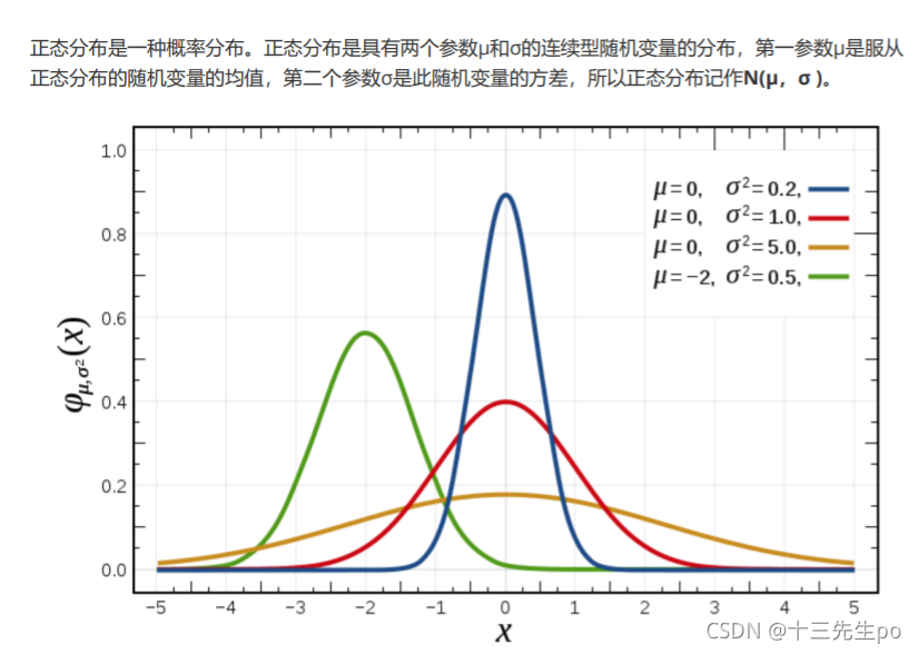
正态分布

• np.random.randn(d0, d1, …, dn)
  功能：从标准正态分布中返回一个或多个样本值
• np.random.normal(loc=0.0, scale=1.0, size=None)
  loc：float
  此概率分布的均值（对应着整个分布的中心centre）
  scale：float
  此概率分布的标准差（对应于分布的宽度，scale越大越矮胖，scale越小，越瘦高）
  size：int or tuple of ints
  输出的shape，默认为None，只输出一个值
• np.random.standard_normal(size=None)
  返回指定形状的标准正态分布的数组。

# 基本操作
# 生成数组的方法
# 4 生成随机数组
# 正态分布
x2 = np.random.normal(1.75,1,10000000)
x2

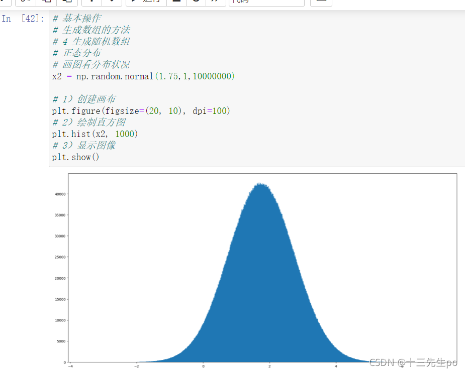
• 画图看分布状况

# 基本操作
# 生成数组的方法
# 4 生成随机数组
# 正态分布
# 画图看分布状况
x2 = np.random.normal(1.75,1,10000000)

# 1）创建画布
plt.figure(figsize=(20, 10), dpi=100)
# 2）绘制直方图
plt.hist(x2, 1000)
# 3）显示图像
plt.show()

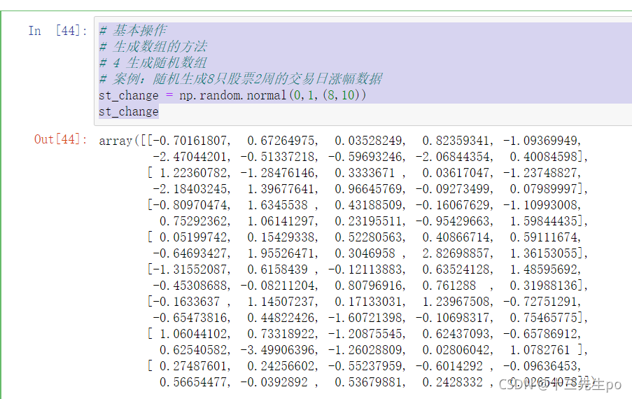
案例：随机生成8只股票2周的交易日涨幅数据

8只股票，两周(10天)的涨跌幅数据，如何获取？

• 两周的交易日数量为：2 X 5 =10
• 随机生成涨跌幅在某个正态分布内，比如均值0，方差1

# 基本操作
# 生成数组的方法
# 4 生成随机数组
# 案例：随机生成8只股票2周的交易日涨幅数据
st_change = np.random.normal(0,1,(8,10))
st_change

3.1.2 数组值的改变

# 基本操作
# 生成数组的方法
# 生成0和1的数组
one = np.ones([3,4])
one[1] = 3
one

# 基本操作
# 生成数组的方法
# 2 从现有数组生成
a = np.array([[1,2,3],[4,5,6]])
a[1] = 4
print(a)
print(a.dtype)
print('============')
# 从现有的数组当中创建
a1 = np.array(a)
print(a1)
print(a1.dtype)
print('============')
# 相当于索引的形式，并没有真正的创建一个新的
a2 = np.asarray(a)
print(a2)
print(a2.dtype)

3.1.3 数组的索引、切片

目标代码

st_change = np.random.normal(0,1,(8,10))
st_change

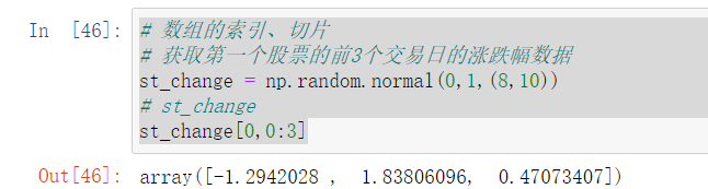
• 获取第一个股票的前3个交易日的涨跌幅数据

# 数组的索引、切片
# 获取第一个股票的前3个交易日的涨跌幅数据
st_change = np.random.normal(0,1,(8,10))
# st_change
st_change[0,0:3]

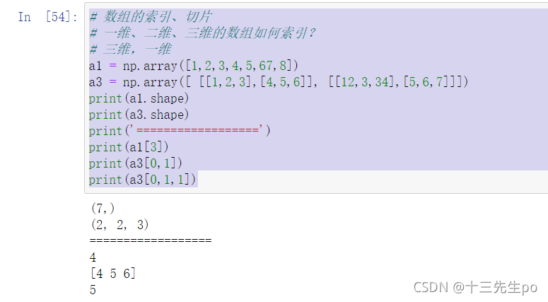
一维、二维、三维的数组如何索引？

# 数组的索引、切片
# 一维、二维、三维的数组如何索引？
# 三维，一维
a1 = np.array([1,2,3,4,5,67,8])
a3 = np.array([ [[1,2,3],[4,5,6]], [[12,3,34],[5,6,7]]])
print(a1.shape)
print(a3.shape)
print('==================')
print(a1[3])
print(a3[0,1])
print(a3[0,1,1])

3.1.4 形状修改

需求：让刚才的股票行、日期列反过来，变成日期行，股票列

st_change = np.random.normal(0,1,(8,10))
st_change

ndarray.reshape(shape[, order]) Returns an array containing the same data with a new shape

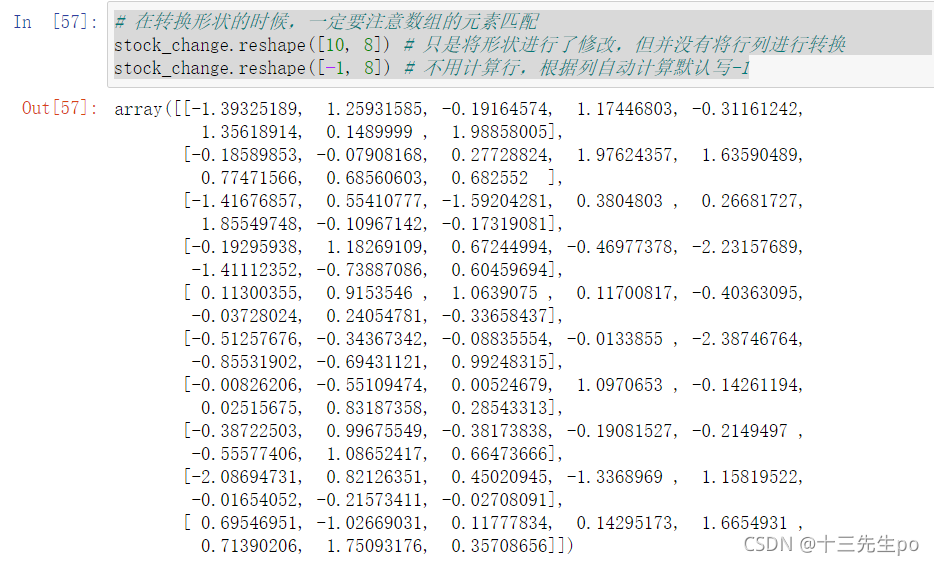
# 在转换形状的时候，一定要注意数组的元素匹配
stock_change.reshape([10, 8]) # 只是将形状进行了修改，但并没有将行列进行转换
stock_change.reshape([-1, 8]) # 不用计算行，根据列自动计算默认写-1

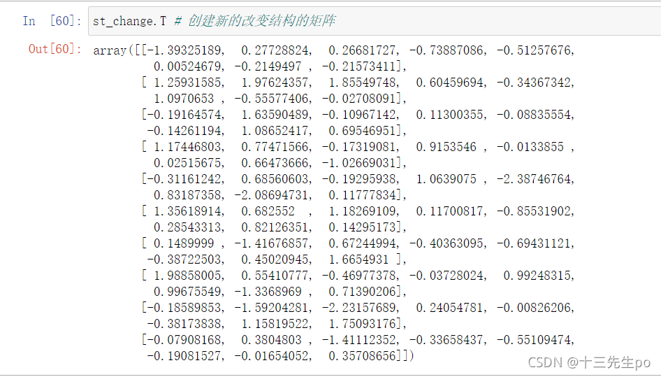
ndarray.T 数组的转置

将数组的行、列进行互换

st_change.T # 创建新的改变结构的矩阵

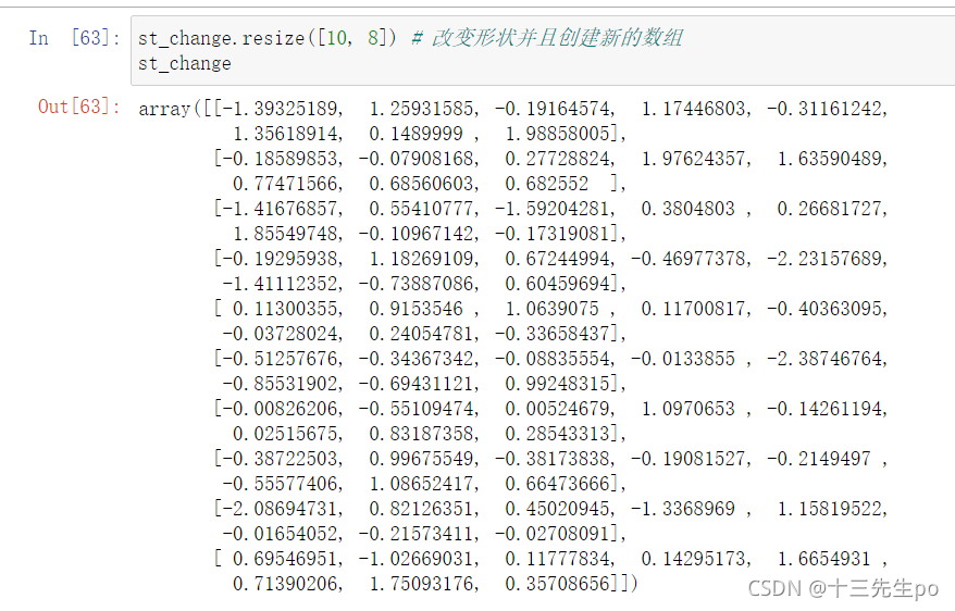
ndarray.resize(new_shape[, refcheck]) Change shape and size of array in-place.

st_change.resize([10, 8]) # 改变形状并且创建新的数组
st_change

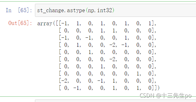
3.1.5 类型修改

ndarray.astype(type)

st_change.astype(np.int32)

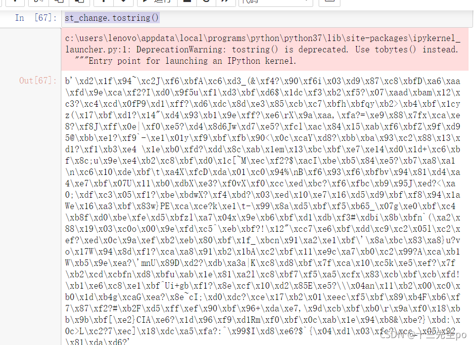
ndarray.tostring([order])或者ndarray.tobytes([order])

Construct Python bytes containing the raw data bytes in the array
转换成bytes

st_change.tostring()

• 拓展：如果遇到

IOPub data rate exceeded.
The notebook server will temporarily stop sending output
to the client in order to avoid crashing it.
To change this limit, set the config variable
`--NotebookApp.iopub_data_rate_limit`.

这个问题是在jupyer当中对输出的字节数有限制，需要去修改配置文件
创建配置文件

jupyter notebook --generate-config
vi ~/.jupyter/jupyter_notebook_config.py

取消注释,多增加

## (bytes/sec) Maximum rate at which messages can be sent on iopub before they
# are limited.
c.NotebookApp.iopub_data_rate_limit = 10000000

但是不建议这样去修改，jupyter输出太大会崩溃

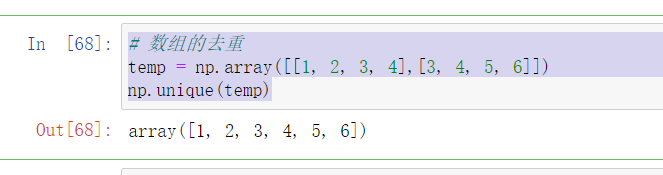
3.1.6 数组的去重

• ndarray.unique

# 数组的去重
temp = np.array([[1, 2, 3, 4],[3, 4, 5, 6]])
np.unique(temp)

3.1.7 小结

• 创建数组
  • 均匀
  • 随机（正态分布）
• 正态分布
• 数组索引
• 数组形状改变
• 数组类型
  • reshape
  • resize
• 数组转换
  • T
  • tostring
  • unique

4 ndarray运算

应用：操作符合某一条件的数据

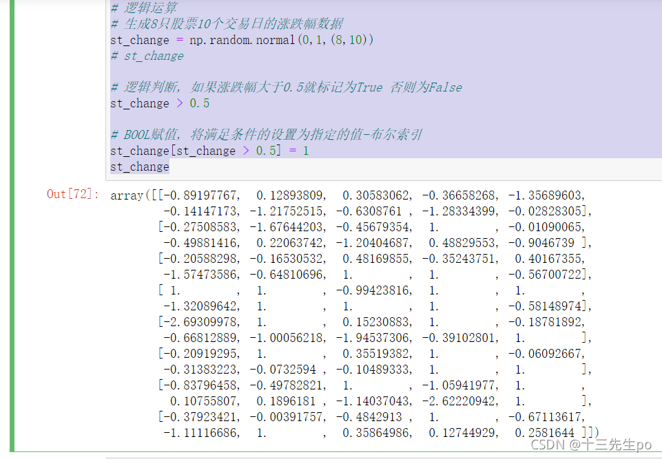
1 逻辑运算

# ndarray运算
# 逻辑运算
# 生成8只股票10个交易日的涨跌幅数据
st_change = np.random.normal(0,1,(8,10))
# st_change

# 逻辑判断, 如果涨跌幅大于0.5就标记为True 否则为False
st_change > 0.5

# BOOL赋值, 将满足条件的设置为指定的值-布尔索引
st_change[st_change > 0.5] = 1
st_change

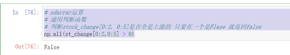
2 通用判断函数

• np.all()

# ndarray运算
# 通用判断函数
# 判断stock_change[0:2, 0:5]是否全是上涨的 只要有一个是Flase 就返回false
np.all(st_change[0:2,0:5] > 0)

• np.any()

# ndarray运算
# 通用判断函数
# 判断前5只股票这段期间是否有上涨的 要有一个是Trye 就返回true
np.all(st_change[0:5,:] > 0) # 写法1
np.all(st_change[0:5] > 0) # 写法2

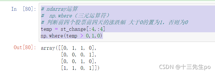
3 np.where（三元运算符）

通过使用np.where能够进行更加复杂的运算

• np.where()

# ndarray运算
#  np.where（三元运算符）
# 判断前四个股票前四天的涨跌幅 大于0的置为1，否则为0
temp = st_change[:4,:4]
np.where(temp > 0,1,0)

• 复合逻辑需要结合np.logical_and和np.logical_or使用

# ndarray运算
#  np.where（三元运算符）
# 复合逻辑需要结合np.logical_and和np.logical_or使用

# 判断前四个股票前四天的涨跌幅 大于0.5并且小于1的，换为1，否则为0
np.where(np.logical_and(temp>0.5,temp<1),1,0)
# 判断前四个股票前四天的涨跌幅 大于0.5或者小于-0.5的，换为1，否则为0
np.where(np.logical_or(temp>0.5,temp<-0.5),1,0)

4 统计运算

想要知道涨幅或者跌幅最大的数据

4.4.1 统计指标

在数据挖掘/机器学习领域，统计指标的值也是我们分析问题的一种方式。常用的指标如下：

• min(a[, axis, out, keepdims])
  -Return the minimum of an array or minimum along an axis.
• max(a[, axis, out, keepdims])
  -Return the maximum of an array or maximum along an axis.
• median(a[, axis, out, overwrite_input, keepdims])
  -Compute the median along the specified axis.
• mean(a[, axis, dtype, out, keepdims])
  -Compute the arithmetic mean along the specified axis.
• std(a[, axis, dtype, out, ddof, keepdims])
  -Compute the standard deviation along the specified axis.
• var(a[, axis, dtype, out, ddof, keepdims])
  -Compute the variance along the specified axis.

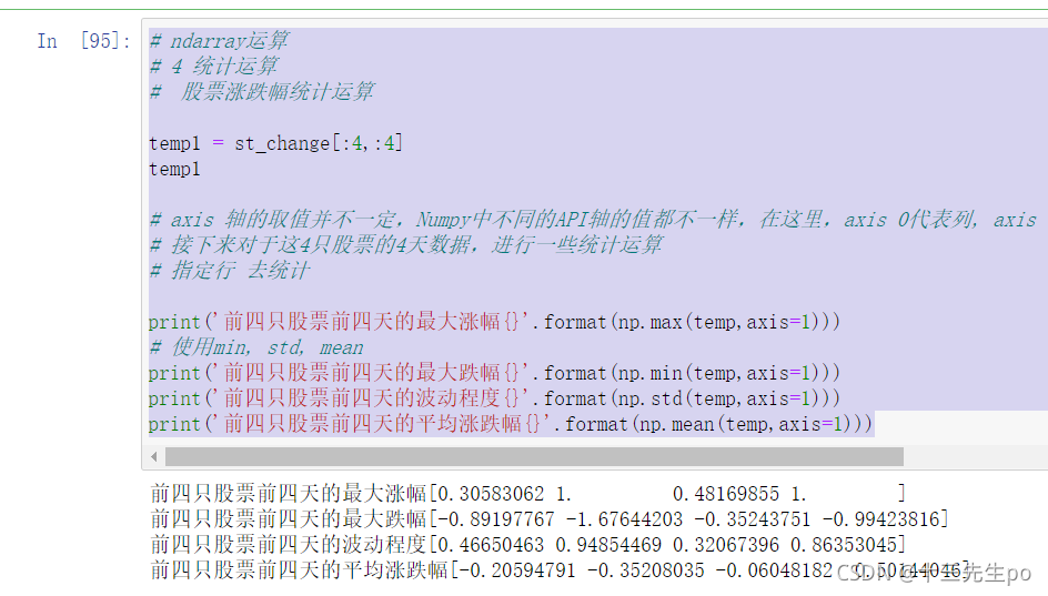
4.4.2 股票涨跌幅统计运算

进行统计的时候，axis 轴的取值并不一定，Numpy中不同的API轴的值都不一样，在这里，axis 0代表列, axis 1代表行去进行统计

# ndarray运算
# 4 统计运算
#  股票涨跌幅统计运算

temp1 = st_change[:4,:4]
temp1

# axis 轴的取值并不一定，Numpy中不同的API轴的值都不一样，在这里，axis 0代表列, axis 1代表行去进行统计
# 接下来对于这4只股票的4天数据，进行一些统计运算
# 指定行 去统计

print('前四只股票前四天的最大涨幅{}'.format(np.max(temp,axis=1)))
# 使用min, std, mean
print('前四只股票前四天的最大跌幅{}'.format(np.min(temp,axis=1)))
print('前四只股票前四天的波动程度{}'.format(np.std(temp,axis=1)))
print('前四只股票前四天的平均涨跌幅{}'.format(np.mean(temp,axis=1)))

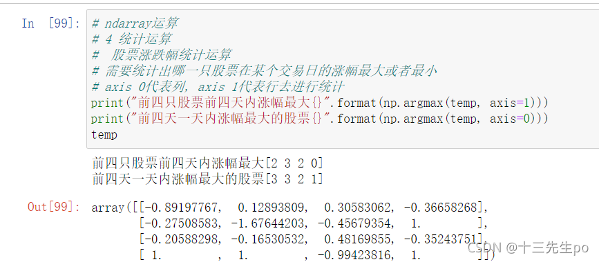
• 需要统计出哪一只股票在某个交易日的涨幅最大或者最小
  • np.argmax(temp, axis=)
  • np.argmin(temp, axis=)

# ndarray运算
# 4 统计运算
#  股票涨跌幅统计运算
# 需要统计出哪一只股票在某个交易日的涨幅最大或者最小
print("前四只股票前四天内涨幅最大{}".format(np.argmax(temp, axis=1)))
print("前四天一天内涨幅最大的股票{}".format(np.argmax(temp, axis=0)))
temp

4.4.3 sum()求和、np.bincount(xx)分类频率计数

适用于一维数组的所有值相加

• sum()求和

目标数组

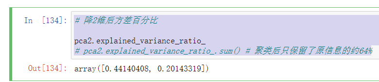
# 降2维后方差百分比

pca2.explained_variance_ratio_
# pca2.explained_variance_ratio_.sum() # 聚类后只保留了原信息的约64%

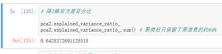
进行求和

# 降2维后方差百分比

pca2.explained_variance_ratio_
pca2.explained_variance_ratio_.sum() # 聚类后只保留了原信息的约64%

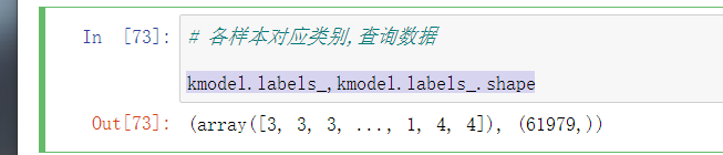
• np.bincount(xx) 分类频率计数
  可以认为是一维数组的分类聚合

目标数据，有61979条

kmodel.labels_,kmodel.labels_.shape

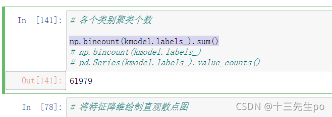
进行求和

np.bincount(kmodel.labels_)

加起来的数量也没有变化

np.bincount(kmodel.labels_).sum()

5 数组间的运算

1 应用背景

[[80, 86],
[82, 80],
[85, 78],
[90, 90],
[86, 82],
[82, 90],
[78, 80],
[92, 94]]

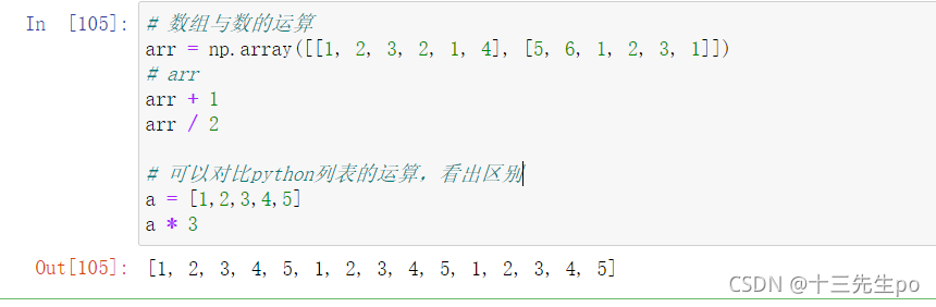
2 数组与数的运算

# 数组与数的运算
arr = np.array([[1, 2, 3, 2, 1, 4], [5, 6, 1, 2, 3, 1]])
# arr
arr + 1
arr / 2

# 可以对比python列表的运算，看出区别
a = [1,2,3,4,5]
a * 3

但是下面这个数组直接运算是不行的

# 数组与数的运算
# 错误示范
arr1 = np.array([[1, 2, 3, 2, 1, 4], [5, 6, 1, 2, 3, 1]])
arr2 = np.array([[1, 2, 3, 4], [3, 4, 5, 6]])

arr1 + arr2

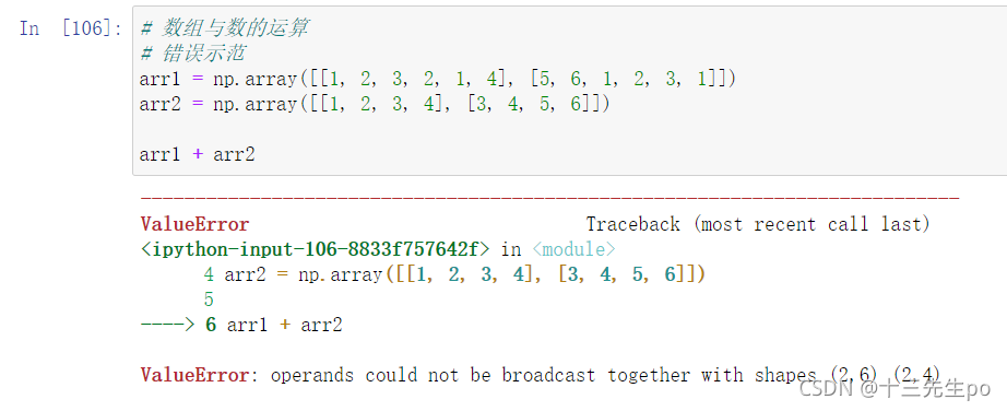
报错：

ValueError: operands could not be broadcast together with shapes (2,6) (2,4) 

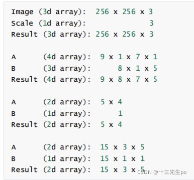
3 广播机制

执行 broadcast 的前提在于，两个 ndarray 执行的是 element-wise的运算，Broadcast机制的功能是为了方便不同形状的ndarray（numpy库的核心数据结构）进行数学运算。
当操作两个数组时，numpy会逐个比较它们的shape（构成的元组tuple），只有在下述情况下，两个数组才能够进行数组与数组的运算。

• 维度相等
• shape（其中相对应的一个地方为1）

广播机制如果简单理解的话，就是看一个数组能否扩展为另一个数组的结构，以便他们之间能进行运算

• 例如，一个三行两列的数组，和一个一行2列的数组，或一个单值数组，后两个都可以广播扩展为三行两列，就可以进行计算

上面的讲解就一个理解为

• 1可以变成任意多个值
• 一，或者相同个数，都可以广播
  以下例子都可以进行运算

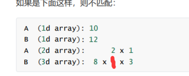
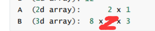
如果是下面这样，则不匹配：

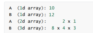
• 10和12不相同，不能运算
• 2和4不相同，不能运算，如果4变成2或者1（合理即可）的话就能运算了
  
  
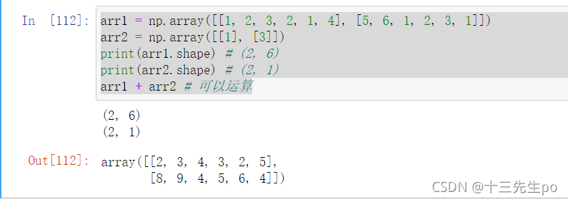
  思考：下面两个ndarray是否能够进行运算？

arr1 = np.array([[1, 2, 3, 2, 1, 4], [5, 6, 1, 2, 3, 1]])
arr2 = np.array([[1], [3]])

答案是可以运算的

arr1 = np.array([[1, 2, 3, 2, 1, 4], [5, 6, 1, 2, 3, 1]])
arr2 = np.array([[1], [3]])
print(arr1.shape) # (2, 6)
print(arr2.shape) # (2, 1)
arr1 + arr2 # 可以运算

4 矩阵运算

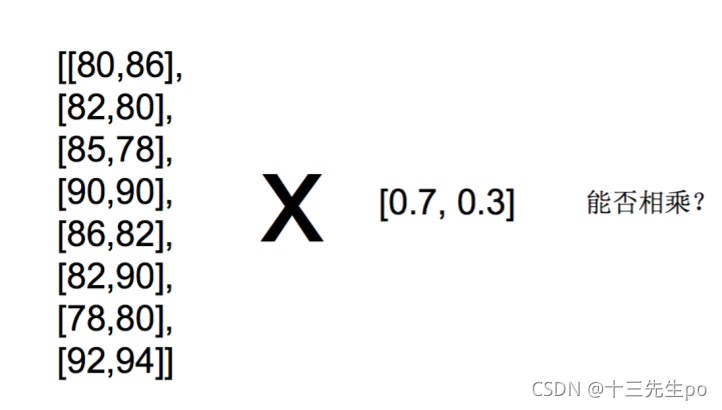
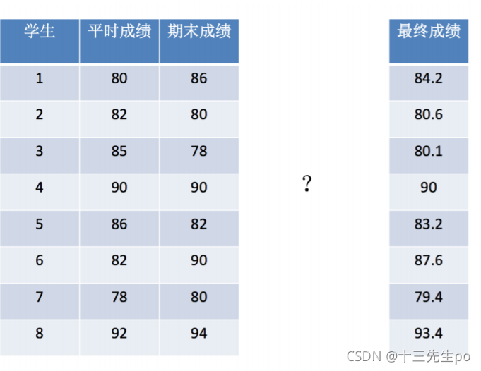
思考：如何能够直接得出每个学生的成绩？

1 什么是矩阵

矩阵，英文matrix，和array的区别矩阵必须是2维的，但是array可以是多维的。
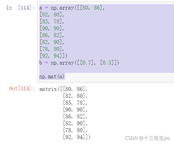
- np.mat()
将数组转换成矩阵类型

# 矩阵运算
# 将数组转换成矩阵类型
a = np.array([[80, 86],
[82, 80],
[85, 78],
[90, 90],
[86, 82],
[82, 90],
[78, 80],
[92, 94]])
b = np.array([[0.7], [0.3]])

np.mat(a)

2 矩阵乘法运算

矩阵乘法的两个关键：

• 形状改变
• 运算规则

形状改变：

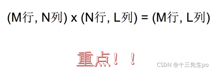
必须符合上面的式子，否则运算出错。
运算规则：

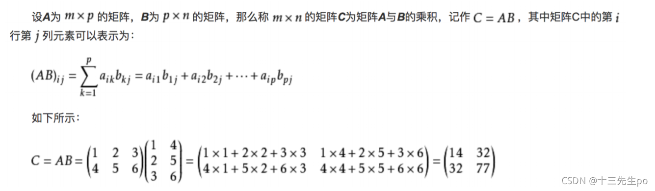
• 矩阵乘法api：
  • np.matmul
  • np.dot

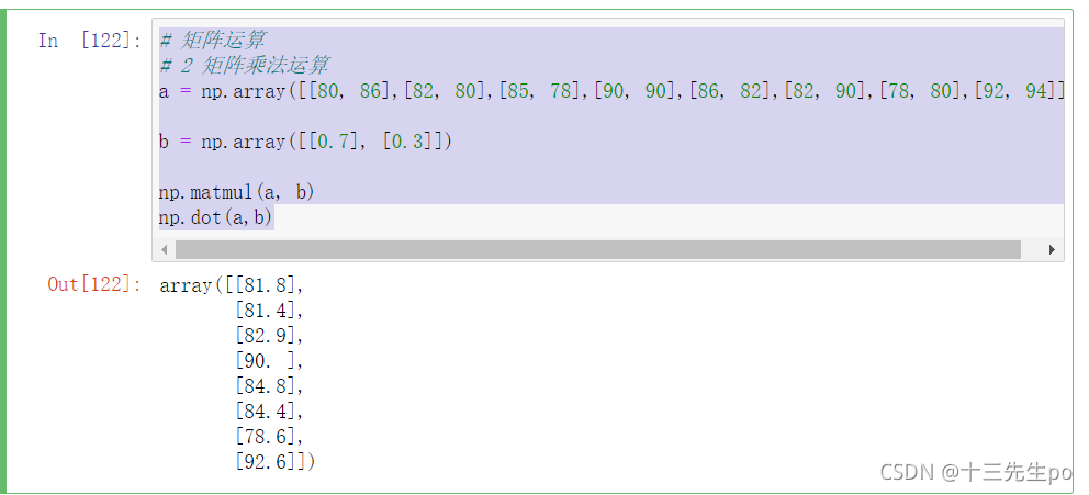
# 矩阵运算
# 2 矩阵乘法运算
a = np.array([[80, 86],[82, 80],[85, 78],[90, 90],[86, 82],[82, 90],[78, 80],[92, 94]])
    
b = np.array([[0.7], [0.3]])

np.matmul(a, b)
np.dot(a,b)

3 矩阵应用场景

大部分机器学习算法需要用到

6 合并、分割

合并、分割的用处：实现数据的切分和合并，将数据进行切分合并处理

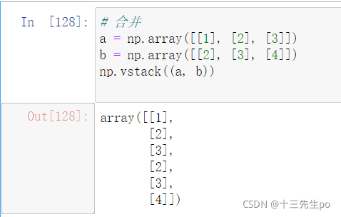
6.1 合并

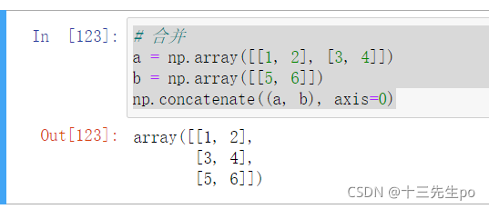
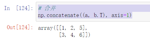
• numpy.concatenate((a1, a2, …), axis=0)
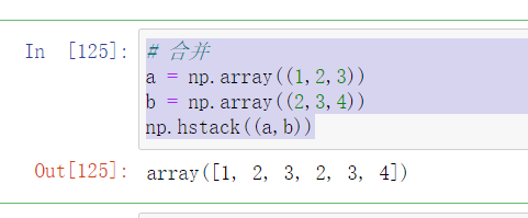
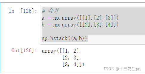
• numpy.hstack(tup) Stack arrays in sequence horizontally (column wise).
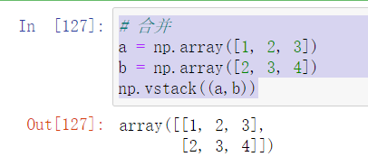
• numpy.vstack(tup) Stack arrays in sequence vertically (row wise).

# 合并
a = np.array([[1, 2], [3, 4]])
b = np.array([[5, 6]])
np.concatenate((a, b), axis=0)

# 合并
np.concatenate((a, b.T), axis=1)

# 合并
a = np.array((1,2,3))
b = np.array((2,3,4))
np.hstack((a,b))

# 合并
a = np.array([[1],[2],[3]])
b = np.array([[2],[3],[4]])

np.hstack((a,b))

# 合并
a = np.array([1, 2, 3])
b = np.array([2, 3, 4])
np.vstack((a,b))

a = np.array([[1], [2], [3]])
b = np.array([[2], [3], [4]])
np.vstack((a, b))

比如我们将两部分股票的数据拼接在一起：

# 比如我们将两部分股票的数据拼接在一起：
a = st_change[:2,0:4]
b = st_change[4:6,0:4]
a
b
# axis=1时候，按照数组的列方向拼接在一起
# axis=0时候，按照数组的行方向拼接在一起
print(np.concatenate([a,b],axis=1))
print(np.hstack([a,b]))
print('============================')
print(np.concatenate([a,b],axis=0))
print(np.vstack([a,b]))

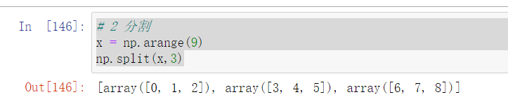
6.2 分割

• numpy.split(ary, indices_or_sections, axis=0)
  Split an array into multiple sub-arrays.

# 2 分割
# 按间隔分
x = np.arange(9)
np.split(x,3)

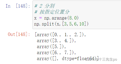
# 2 分割
# 按指定位置分
x = np.arange(8.0)
np.split(x,[3,5,6,10])

7 IO操作与数据

7.1 问题

大多数数据并不是我们自己构造的，而是存在文件当中，需要我们用工具获取。
但是Numpy其实并不适合用来读取和处理数据，因此我们这里了解相关API，以及Numpy不方便的地方即可。

7.2 Numpy读取

• genfromtxt(fname[, dtype, comments, …])
  Load data from a text file, with missing values handled as specified.
  

# 读取数据
test = np.genfromtxt("test.csv", delimiter=',')

7.3 如何处理缺失值

1 什么是缺失值

什么时候numpy中会出现nan：当我们读取本地的文件为float的时候，如果有缺失(或者为None)，就会出现nan

2 缺失值处理

那么，在一组数据中单纯的把nan替换为0，合适么？会带来什么样的影响？

比如，全部替换为0后，替换之前的平均值如果大于0，替换之后的均值肯定会变小，所以更一般的方式是把缺失的数值替换为均值（中值）或者是直接删除有缺失值的一行

所以：

• 如何计算一组数据的中值或者是均值
• 如何删除有缺失数据的那一行（列）在pandas中介绍