Tensorflow笔记——神经网络图像识别（四）搭建模块化的神经网络八股（正则化，指数衰减学习率，滑动平均等优化）

实战案例：

数据X【x0，x1】为正太分布随机点，

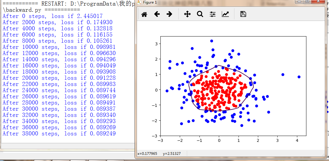
标注Y_，当x0*x0+x1*x1<2时，y_=1（红），否则y_=0(蓝)

建立三个.py文件

1. generateds.py生成数据集

import numpy as np
import matplotlib.pyplot as plt
seed = 2
def generateds():
    #基于seed产生随机数
    rdm = np.random.RandomState(seed)
    #随机数返回200列2行的矩阵，表示300组坐标点（x0，x1）作为输入数据集
    X = rdm.randn(300,2)
    #如果X中的2个数的平方和<2，y=1,否则y=2
    #作为输入数据集的标签（正确答案）
    Y_ = [int(x0*x0 + x1*x1 <2) for (x0,x1) in X]
    #为方便可视化，遍历Y_中的每个元素，1为红，0为蓝
    Y_c = [['red' if y else 'blue'] for y in Y_]
    #对数据集X和标签Y进行形状整理，-1表示n，n行2列写为reshape(-1,2)
    X = np.vstack(X).reshape(-1,2)
    Y_ = np.vstack(Y_).reshape(-1,1)
    #print(X)
    #print(Y)
    #print(Y_c)
    return X,Y_,Y_c

'''
if __name__ == '__main__':
    X,Y_,Y_c=generateds()

    #用 plt.scatter画出数据集X中的点（x0.x1），Y_c表示颜色
    plt.scatter(X[:,0], X[:,1],c=np.squeeze(Y_c))
    plt.show()
'''

2. forward.py 前向传播

#coding:utf-8
import tensorflow as tf

#定义神经网络的输入、参数和输出，定义前项传播过程
def get_weight(shape, regularizer):
    w = tf.Variable(tf.random_normal(shape),dtype=tf.float32)
    #把每个w的正则化损失加到总损失losses中
    tf.add_to_collection('losses', tf.contrib.layers.l2_regularizer(regularizer)(w))
    return w

def get_bias(shape):
    b=tf.Variable(tf.constant(0.01, shape=shape))
    return b

#搭建前向传播框架
def forward(x, regularizer):

    w1 = get_weight([2,11], regularizer)
    b1 = get_bias([11])
    #(x和w1实现矩阵乘法 + b1)过非线性函数（激活函数）
    y1 = tf.nn.relu(tf.matmul(x, w1) + b1)

    w2 = get_weight([11,1], regularizer)
    b2 = get_bias([1])
    #输出层不过激活函数
    y = tf.matmul(y1, w2) + b2

    return y

3. backward.py 反向传播

#coding:utf-8
import tensorflow as tf
import numpy as np
import matplotlib.pyplot as plt
import generateds
import forward

STEPS = 40000#共进行40000轮
BATCH_SIZE = 30#表示一次为喂入NN多少组数据
LEARNING_RATE_BASE = 0.001#学习率基数，学习率初始值
LEARNING_RATE_DECAY = 0.999#学习率衰减率
REGULARIZER = 0.01#参数w的loss在总losses中的比例，即正则化权重

def backward():
    x = tf.placeholder(tf.float32,(None,2))
    y_ = tf.placeholder(tf.float32,(None,1))

    X,Y_,Y_c = generateds.generateds()

    y=forward.forward(x, REGULARIZER)

    global_step = tf.Variable(0, trainable = False)

    learning_rate = tf.train.exponential_decay(
        LEARNING_RATE_BASE,
        global_step,300/BATCH_SIZE,
        LEARNING_RATE_DECAY,
        staircase = True)

    #定义损失函数
    loss_mse = tf.reduce_mean(tf.square(y-y_))#利用均方误差
    loss_total = loss_mse + tf.add_n(tf.get_collection('losses'))

    #定义反向传播方法：包含正则化
    train_step = tf.train.AdamOptimizer(learning_rate).minimize(loss_total)

    with tf.Session() as sess :
        init_op = tf.global_variables_initializer()
        sess.run(init_op)
        for i in range(STEPS):
            start =(i*BATCH_SIZE) % 300
            end = start + BATCH_SIZE
            sess.run(train_step, feed_dict={x:X[start:end], y_:Y_[start:end]})
            if i % 2000 == 0:
                loss_v = sess.run(loss_total, feed_dict={x:X,y_:Y_})
                print('After %d steps, loss if %f '%(i,loss_v))

            #xx在-3到3之间步长为0.01，yy在-3到3之间步长为0.01生成二维网格坐标点 
            xx, yy = np.mgrid[-3:3.01, -3:3:.01]
            #将xx，yy拉直，并合并成一个2列的矩阵，得到一个网格坐标点的集合
            grid = np.c_[xx.ravel(), yy.ravel()]
            #将网格坐标点喂入神经网络，probs为输出
            probs = sess.run(y, feed_dict={x:grid})
            #将probs的shape调整成xx的样子
            probs = probs.reshape(xx.shape)

        #画出离散点
        plt.scatter(X[:,0], X[:,1], c=np.squeeze(Y_c))
        #画出probs，0.5的曲线
        plt.contour(xx, yy, probs, levels=[.5])
        plt.show()

if __name__ == '__main__':
    backward()

输出：

如果对你有帮助，欢迎打赏！

Tensorflow笔记——神经网络图像识别（四）搭建模块化的神经网络八股（正则化，指数衰减学习率，滑动平均等优化）

猜你喜欢