@article{rosasco2004are,
title={Are loss functions all the same},
author={Rosasco, Lorenzo and De Vito, Ernesto and Caponnetto, Andrea and Piana, Michele and Verri, Alessandro},
journal={Neural Computation},
volume={16},
number={5},
pages={1063--1076},
year={2004}}
概
作者给出了不同的损失函数, 在样本数量增多情况下的极限情况. 假设\(p(x,y)\)为\((x,y)\)的密度函数,其中\(x\in \mathbb{R}^d\)为输入样本, \(y\in \mathbb{R}\)为值(回归问题) 或 类别信息(分类问题). 设\(V(w,y),\)为损失函数, 则期望风险为:
\[ \tag{1} I[f]=\int_Z V(f(x),y)p(x,y)\mathrm{d} x \mathrm{d}y, \]
其中\(f\)为预测函数, 不妨设\(f_0\)最小化期望风险. 在实际中, 我们只有有限的样本\(D=\{(x_1,y_1),\ldots, (x_l,y_l)\}\), 在此情况下, 我们采取近似
\[ \tag{2} I_{emp}[f]=\frac{1}{l}\sum_{i=1}^lV(f(x_i),y_i), \]
同时
\[ \tag{3} f_D=\arg\min_{f \in \mathcal{H}} I_{emp}[f]. \]
其中\(\mathcal{H}\)为hypothesis space.
\(f_D\)与\(f_0\)之间的差距如何, 是本文的核心.
主要内容
一些假设
首先\(f_D\)的在空间\(\mathcal{H}\)中寻找, Reproducing Kernel Hilbert Space(RKHS)一文中(没看)给出了这种空间的构造方式. 给定对称正定函数\(K(x,s)\)(Mercer核):
\[ K: X \times X \rightarrow \mathbb{R}, \]
同时\(K(\cdot, x)\)是连续函数.
函数\(f\)通过下述方式构造:
\[ \tag{4} f(x) = \langle f, K(\cdot, x)\rangle_{\mathcal{H}}. \]
给定常数\(R>0\), 构造hypothesis space \(\mathcal{H}_{R}\):
\[ \mathcal{H}_{R} = \{f \in \mathcal{H}, \|f\|_{\mathcal{H}}\le R\}, \]
则在\(\|\cdot\|_{\infty}\)下, \(\mathcal{H}_R\)是连续函数\(C(X)\)上的一个紧集,其中\(X\subset \mathbb{R}^d\)是紧的(这个证明要用到经典的Arela-Ascoli定理, 只需证明\(\mathcal{H}_R\)中的元素是等度连续即可).
另外:
\[ |f(x)|= |\langle f, K(\cdot, x)\rangle_{\mathcal{H}}.| \le \|f\|_{\mathcal{H}} \sqrt{K(x,x)}, \]
故
\[ \|f(x)\|_{\infty} \le RC_K, \]
其中\(C_K=\sup_{x \in X} \sqrt{K(x,x)}\).
损失函数\(V\)为凸函数且满足:
- \(V\)是Lipschitz函数, 即对于任意的\(M>0\), 存在常数\(L_M>0\)使得
\[ |V(w_1,y)-V(w_2,y)|\le L_M|w_1-w_2|, \]对于任意的\(w_1,w_2\in[-M,M],y\in Y\)成立. - 存在常数\(C_0\), \(\forall y\in Y\)
\[ V(0, y) \le C_0, \]
成立.
注: 这里的凸函数, 因为一般的损失函数实际上是以\(w-y\)(回归), \(wy\)(分类)为变元, 所以要求\(V(t)\)关于\(t=w-y\)或者\(t=wy\)为凸函数.
损失函数
回归问题:

分类问题:
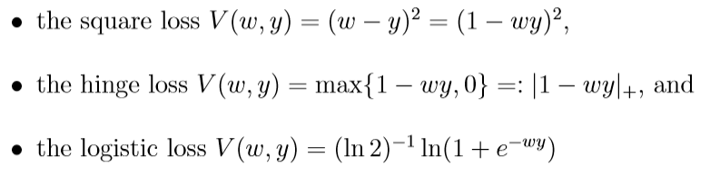
这些损失函数都是满足假设的, 所对应的\(L_M, C_0\), 当\(Y=[a, b], \delta=\max \{|a|, |b|\}\)时为

\(I[f_D]-I[f_R]\)
假设\(f_R=\arg\min_{f \in \mathcal{H}_R}I[f]\), 一般的误差
\[ I[f_D]-I[f_0]=(I[f_D]-I[f_R])+(I[f_R]-I[f_0]), \]
第一项是我们所关注的, 称为估计误差, 第二项为逼近误差.
这里引入\(\mathcal{H}_R\)的covering number, \(N(\epsilon)\), 文中所指的应该是wiki中的external covering number.
下面是理论结果, 引理的证明用了Hoeffding不等式, 这个不了解, 感兴趣请回看原文.
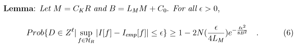

这里\(\epsilon(\eta, \ell, R)\)实际上(6)不等式右端第二项, 令其为\(\eta\), 反解\(\epsilon\)的意思.
第一个不等式实际上就是引理的推论, 第二个不等式注意到:
又\(I[f_D]\ge I[f_R]\)(这个说是根据定义, 但我没弄清楚), 故不等式成立.
损失函数的统计性质
收敛速度
考察不同损失的函数的\(\eta\):
回归问题:
\(abs / \epsilon-insensitive\):
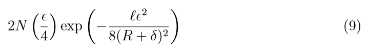
\(square\):
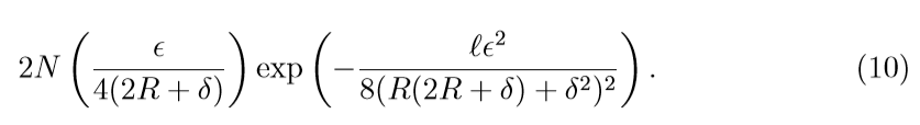
注意到, 因为square loss 的covering number 随着\(R, \delta\)的增加会变大, 所以\(\eta\)会变大,所以在收敛速度上, square比不上上面俩个.

分类问题:
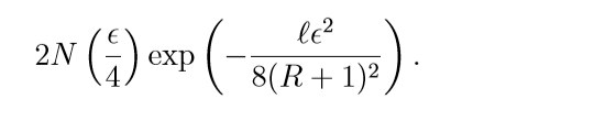
hinge:
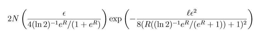
logistic:
二者的收敛表现是类似的, 而square是类似的(\(\delta=1\)).
分类的界
关注分类问题中的hinge损失, 因为它会逼近概率推断.
在二元分类问题中, 其最佳函数\(f_b\)为:
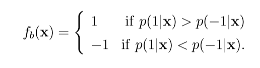
当\(p(1|x)\not= p(-1|x)\).
有如下事实:

证明蛮有趣的, 这里贴一下

\(p(1|x)<1/2\)的证明是类似的.
另外(证明在别的论文中):
\[ \tag{11}I[f_0]=I[f_b]. \]
又(至少有\(1-\eta\)的概率)
\[ I[f_D]-I[f_R]\le2\epsilon(\eta, \ell, R), \]
并注意到(感觉怪怪的):
\[ I[sgn(f_D)] \le I[f_D], \]
故至少有\(1-\eta\)的概率
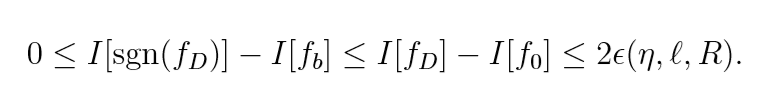
成立. 也就是说当样本个数\(\ell\)足够大的时候, \(sgn(f_D)\)的效用是等价于统计判别的, 这是hinge loss独有的优势.