一、学习“梯度下降法”
1、推荐学习链接:(简书)深入浅出–梯度下降法及其实现
2、结合链接中代码补充代码(主要添加了绘图)如下:
import numpy as np
import matplotlib.pyplot as plt
# Size of the points dataset.
m = 20

# Points x-coordinate and dummy value (x0, x1).
X0 = np.ones((m, 1))
X1 = np.arange(1, m+1).reshape(m, 1)
X = np.hstack((X0, X1))

# Points y-coordinate
y = np.array([
    3, 4, 5, 5, 2, 4, 7, 8, 11, 8, 12,
    11, 13, 13, 16, 17, 18, 17, 19, 21
]).reshape(m, 1)
'''
plt.plot(X1,y)
plt.show()
plt.scatter(X1,y)
plt.show()
'''
# The Learning Rate alpha.
alpha = 0.01

def error_function(theta, X, y):
    '''Error function J definition.(误差函数J)'''
    diff = np.dot(X, theta) - y
    return (1./2*m) * np.dot(np.transpose(diff), diff)

def gradient_function(theta, X, y):
    '''Gradient of the function J definition..(误差函数J梯度定义,对theta求导结果)'''
    diff = np.dot(X, theta) - y
    return (1./m) * np.dot(np.transpose(X), diff)

def gradient_descent(X, y, alpha):
    '''Perform gradient descent.'''
    theta = np.array([1, 1]).reshape(2, 1)
    gradient = gradient_function(theta, X, y) #梯度下降最快的方向
    while not np.all(np.absolute(gradient) <= 1e-5):
        theta = theta - alpha * gradient
        gradient = gradient_function(theta, X, y)
    return theta

optimal = gradient_descent(X, y, alpha)
print('optimal:', optimal)
print('error function:', error_function(optimal, X, y)[0,0])
#绘制拟合后的图形和散点图
plt.rcParams['font.sans-serif'] = 'SimHei' #用于正常显示中文
plt.title('数据散点图及其梯度下降法拟合出的直线') ## 添加标题
plt.xlabel('x')## 添加x轴的名称
plt.ylabel('y')## 添加y轴的名称
plt.xlim([0,20])## 确定x轴范围
plt.ylim([0,20])## 确定y轴范围
plt.xticks([0,5,10,15,20])## 规定x轴刻度
plt.yticks([0,5,10,15,20])## 确定y轴刻度
plt.plot(X,optimal[0]+optimal[1]*X)
plt.scatter(X1,y)
plt.show()

3、绘制误差函数J的图形(方法有些笨拙,有待改进)
from mpl_toolkits import mplot3d
import matplotlib.pyplot as plt
import numpy as np
plt.rcParams['axes.unicode_minus'] = False ## 设置正常显示符号,主要是负号的显示

a=np.arange(-1,3,0.1)
N=a.size
Z=np.zeros((N,N))

def error_function(theta):
    '''Error function J definition.'''
    m = 20
    X0 = np.ones((m, 1))
    X1 = np.arange(1, m+1).reshape(m, 1)
    X = np.hstack((X0, X1))
    y = np.array([
    3, 4, 5, 5, 2, 4, 7, 8, 11, 8, 12,
    11, 13, 13, 16, 17, 18, 17, 19, 21
    ]).reshape(m, 1)
    diff = np.dot(X, theta) - y
    return (1./2*m) * np.dot(np.transpose(diff), diff)

for i in range(0,N):
    for j in range(0,N):
        theta = np.array([[a[i],a[j]]]).reshape(2, 1)
        Z[i][j]=error_function(theta)


X, Y = np.meshgrid(a,a)
ax = plt.axes(projection='3d')
fig = plt.figure()
#ax = Axes3D(fig)
#ax.plot_surface(X, Y, Z)
#调整观察角度和方位角。这里将俯仰角设为45度,把方位角调整为90度
#ax.view_init(60, 45)
ax.plot_surface(X, Y, Z, rstride=1, cstride=1, cmap='rainbow', edgecolor='none')
①ax = plt.axes(projection=‘3d’)
ax.plot_surface(X, Y, Z)语句绘图结果

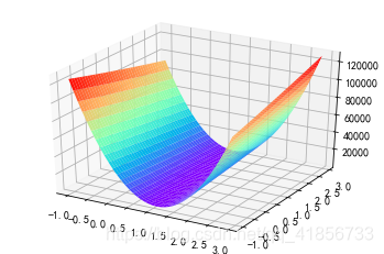
②ax = plt.axes(projection=‘3d’)
ax.plot_surface(X, Y, Z, rstride=1, cstride=1, cmap=‘rainbow’, edgecolor=‘none’)绘图结果:
二、尝试梯度下降法可视化
1、推荐参考链接:
①图解深度学习-梯度下降学习率可视化
②Matplotlib学习笔记——画三维图
2、先记录问题和代码修改的过程
①不知道如何把两个三维图画到一张图里
解决:实际上不需要可以用什么函数把两张图画在一起,不新建一个坐标实际上就会画在一起,感觉没画在一起是因为被挡住了。

倘若把曲面图改成线框图就很容易发现这个问题了

②尝试把z轴方向上的点往上移动一点,但效果不理想
ax.scatter3D(t1, t2, ff(t1,t2)+3, c=‘r’,marker = ‘o’) #往上移动三个单位
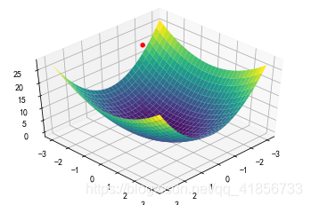
③那就不往上移了,改成登高线图好了

④调整个角度、初始值和迭代次数之后的结果(效果还不错)

3、没有整理的代码
(注意这个代码的可调节变量功能在Spyter中可能不能用,我是在Jupyter Notebook中运行的)
import numpy as np
import matplotlib.pyplot as plt
from ipywidgets import *
from mpl_toolkits import mplot3d #用于绘制3D图形
#梯度函数的导数
def gradJ1(theta):
    return 4*theta
def gradJ2(theta):
    return 2*theta

#梯度函数
def f(x, y):
    return  2*x**2 +y**2

def ff(x,y):
    return 2*np.power(x,2)+np.power(y,2)

def train(lr,epoch,theta1,theta2,up,dirc):
    t1 = [theta1]
    t2 = [theta2]
    for i in range(epoch):
        gradient = gradJ1(theta1)
        theta1 = theta1 - lr*gradient
        t1.append(theta1)
        gradient = gradJ2(theta2)
        theta2 = theta2 - lr*gradient
        t2.append(theta2)

    plt.figure(figsize=(10,10))     #设置画布大小
    x = np.linspace(-3,3,30)
    y = np.linspace(-3,3,30)
    X, Y = np.meshgrid(x, y)
    Z = f(X,Y)
    ax = plt.axes(projection='3d')
    fig =plt.figure()
    #ax1 = plt.subplot(2, 1, 1)
    #ax.plot_surface(X, Y, Z, rstride=1, cstride=1, cmap='viridis', edgecolor='none') #曲面图
    #ax.plot_wireframe(X, Y, Z, color='c') #线框图
    ax.contour3D(X, Y, Z, 50, cmap='binary')#等高线图
    #fig =plt.figure()
    #print(t1)
    #print(ff(t1,t2)+10)
    #ax1 = plt.subplot(2, 2, 1)
    ax.scatter3D(t1, t2, ff(t1,t2), c='r',marker = 'o')
    #ax.plot3D(t1, t2,  ff(t1,t2),'red')
    #调整观察角度和方位角。这里将俯仰角设为60度,把方位角调整为35度
    ax.view_init(up, dirc)

#可以随时调节,查看效果 (最小值,最大值,步长)
@interact(lr=(0, 2, 0.0002),epoch=(1,100,1),init_theta1=(-3,3,0.1),init_theta2=(-3,3,0.1),up=(-180,180,1),dirc=(-180,180,1),continuous_update=False)
#lr为学习率(步长) epoch为迭代次数   init_theta为初始参数的设置 up调整图片上下视角 dirc调整左右视角
def visualize_gradient_descent(lr=0.05,epoch=10,init_theta1=-2,init_theta2=-3,up=45,dirc=100):
    train(lr,epoch,init_theta1,init_theta2,up,dirc)
可调参数及其初始值:

运行效果图:

4、换了个稍微复杂点的函数并简化后的代码:
函数:sin( sqrt(x^2 +y^2))
import numpy as np
import matplotlib.pyplot as plt
from ipywidgets import *         #引进用于调用“变量控制滚动条”的包
from mpl_toolkits import mplot3d #用于绘制3D图形

#梯度函数的导数
def gradJ1(x,y):
    return x / (np.sqrt(x ** 2 + y ** 2)) * np.cos(np.sqrt(x ** 2 + y ** 2))
def gradJ2(x,y):
    return y  / (np.sqrt(x ** 2 + y ** 2)) * np.cos(np.sqrt(x ** 2 + y ** 2))

#梯度函数
def f(x, y):
    return  np.sin(np.sqrt(x ** 2 + y ** 2))

def train(lr,epoch,theta1,theta2,up,dirc):
    #下面的三个数组,由于记录迭代过程的路径
    t1 = [theta1]
    t2 = [theta2]
    z=[f(theta1,theta2)]
    for i in range(epoch):
        gradient = gradJ1(theta1,theta2)
        theta1 = theta1 - lr*gradient
        t1.append(theta1)
        gradient = gradJ2(theta1,theta2)
        theta2 = theta2 - lr*gradient
        t2.append(theta2)
        z.append(f(theta1,theta2))

    plt.figure(figsize=(12,12))     #设置画布大小
    x = np.linspace(-6,6,100)
    y = np.linspace(-6,6,100)
    X, Y = np.meshgrid(x, y)
    Z = f(X,Y)
    ax = plt.axes(projection='3d')
    ax.contour3D(X, Y, Z, 50, cmap='binary')#等高线图
    ax.scatter3D(t1, t2, z, c='r',marker = 'o')#散点图
    #调整观察角度和方位角。这里将俯仰角设为45度,把方位角调整为45度
    ax.view_init(up, dirc)

#可以随时调节,查看效果 (最小值,最大值,步长) 具体关于ipywidgets包详细怎么用可自行搜索,若只是想简单使用,模仿下面的方式使用即可
@interact(lr=(0, 2, 0.01),epoch=(1,100,1),init_theta1=(-6,6,0.1),init_theta2=(-6,6,0.1),up=(-180,180,1),dirc=(-180,180,1),continuous_update=False)
#lr为学习率(步长) epoch为迭代次数   init_theta为初始参数的设置 up,dirc用于控制视角
def visualize_gradient_descent(lr=0.2,epoch=20,init_theta1=2,init_theta2=0,up=45,dirc=45):
    train(lr,epoch,init_theta1,init_theta2,up,dirc)

补充:init_theta1=1.00,init_theta2=0.50左右,最低点会落在正中心。
5、关于函数求导(求梯度)
上面涉及到一个函数:sin( sqrt(x^2 +y^2))
当然可以直接自己求,但多少有些麻烦,这里推荐一些科学快速求导的方法:
①利用软件(网站求导):
在线求导网站举例
②用Sympy库中的diff的相关函数求导
推荐链接:
@ Python 学习随笔——利用sympy模块中的diff函数来实现对函数的求导
Python 中的Sympy详细使用
import sympy
def func(x,y):
    return sympy.sin(sympy.sqrt(x ** 2 + y ** 2))
x,y = symbols("x,y")
print(diff(func(x,y),x))
运行结果

③SciPy求函数的导数
三、他山之石
1、思路清晰求“梯度下降法”代码
import random
import numpy as np
import matplotlib.pyplot as plt
from mpl_toolkits.mplot3d import Axes3D
def function(x,y):
    z=(x-2)**2+2*(y-1)**2
    return z

#求偏导
def Partial_derivative_fx(x1,x2):
    return 2*(x1-2)
def Partial_derivative_fy(x1,x2):
    return 4*(x2-1)

x1=-10
x2=3

#使用随机数
#x1=random.randint(-10,10)
#x2=random.randint(-10,10)

print(x1,x2)
u = [x1]#x1的数组
v = [x2]#x2的数组
w = [function(x1,x2)]

#梯度下降
k=0#统计次数
a=0.3#步长,0.3和0.4都可以,其他不行
#随机步长
#a=random.random()
print('步长',a)

e=10**(-20)#临界值

while abs(a*Partial_derivative_fx(x1,x2))>e or abs(a*Partial_derivative_fy(x1,x2))>e :
    x1=x1-a*Partial_derivative_fx(x1,x2)
    x2=x2-a*Partial_derivative_fy(x1,x2)
    k=k+1
    u.append(x1)
    v.append(x2)
    w.append(function(x1,x2))
    print(x1,x2)

print(k,'次',function(x1,x2))

#print(u,v)
U = np.array(u)
V = np.array(v)
W = np.array(w)

#画图
fig = plt.figure()
#ax = fig.add_subplot(111, projection='3d')
ax = Axes3D(fig)

X = np.arange(-10, 10, 0.2)
Y = np.arange(-10, 10, 0.2)
X, Y = np.meshgrid(X, Y)

Z = (X-2)**2+2*(Y-1)**2
ax.plot_surface(X, Y, Z, rstride=1, cstride=1, cmap='rainbow')
plt.show()

#画线
ax.scatter(U,V,W,color = 'yellow')
ax.plot(U,V,W,color = 'black')
plt.show()

2、绘制“对比不同学习率收敛速度差异图”的代码
import matplotlib.pyplot as plt
from matplotlib import cm
from mpl_toolkits.mplot3d import Axes3D
import numpy as np
import random

plt.ion()
fig = plt.figure()
ax = fig.gca(projection='3d')

# Make data.
X = np.arange(-4, 4, 0.05)
Y = np.arange(-2, 4, 0.05)
X, Y = np.meshgrid(X,Y)

#原式
Z=(X-2)*(X-2)+2*(Y-1)*(Y-1)

#原函数 分开定义
def Fun(x,y):
    x=x-2
    y=y-1
    x=np.multiply(x,x)
    y=np.multiply(y,y)
    y=y*2
    return x+y
#偏x导
def PxFun(x,y):
    return 2*x-4
#偏y导
def PyFun(x,y):
    return 4*y-4
#代码实现
def steep(x,y,e,ax):
    flag = 1
    k = 0
    while(flag):
        z1 = Fun(x,y)
        x = x - a*PxFun(x,y)
        y = y - a*PyFun(x,y)
        z2 = Fun(x,y)
        if(abs(z1-z2)<e):
            flag=0
        ax.scatter(x,y, Fun(x,y), color='k')
        k=k+1
        if(k>100):
            break
        plt.pause(0.01)

e = 10**(-20)
a = 0.03
surf = ax.plot_surface(X, Y, Z, cmap="rainbow")
ax.set_zlim(0,25)
fig.colorbar(surf, shrink=0.5, aspect=5)

for i in range(3):
    x = random.randint(-1,4)
    y=random.randint(-1,4)
    steep(x,y,e,ax)
plt.show()

A=np.array([0.02,0.04,0.06])

for a in [0.02,0.04,0.06]:
    x=1
    y=3
    flag = 1
    k = 0
    tag_z=[Fun(x,y)]
    tag_k=[0]
    while(flag):
        z1 = Fun(x,y)
        x = x - a*PxFun(x,y)
        y = y - a*PyFun(x,y)
        z2 = Fun(x,y)
        tag_z.append(z2)
        if(abs(z1-z2)<e):
            flag=0
        k=k+1
        tag_k.append(k)
        if(k>50):
            break
    plt.plot(tag_k,tag_z)
plt.title('Objective function,Iterations')
plt.xlabel('Iterations')
plt.ylabel('Objective function')
plt.legend(['a=0.02','a=0.04','a=0.06'])
plt.show()

//2019.11.4更新补充
四、补充一些小技巧
1、在Spyter中图像单独显示的技巧
进行如下设置:
tools——preferences——ipython console——graphics中backend改成automatic或者QT5
设置之后记得重启软件,之后显示的图片就是这样的了:

2、在Jupyter Notebook中显示单独显示图像界面(Spyter亦可)
在代码中加入语句:
%matplotlib auto 或者 %matplotlib qt
若写%matplotlib inline 的图片将不会单独弹出
