《MATLAB 神经网络43个案例分析》：第41章 定制神经网络的实现——神经网络的个性化建模与仿真

1. 前言

《MATLAB 神经网络43个案例分析》是MATLAB技术论坛（www.matlabsky.com）策划，由王小川老师主导，2013年北京航空航天大学出版社出版的关于MATLAB为工具的一本MATLAB实例教学书籍，是在《MATLAB神经网络30个案例分析》的基础上修改、补充而成的，秉承着“理论讲解—案例分析—应用扩展”这一特色，帮助读者更加直观、生动地学习神经网络。

《MATLAB神经网络43个案例分析》共有43章，内容涵盖常见的神经网络（BP、RBF、SOM、Hopfield、Elman、LVQ、Kohonen、GRNN、NARX等）以及相关智能算法（SVM、决策树、随机森林、极限学习机等）。同时，部分章节也涉及了常见的优化算法（遗传算法、蚁群算法等）与神经网络的结合问题。此外，《MATLAB神经网络43个案例分析》还介绍了MATLAB R2012b中神经网络工具箱的新增功能与特性，如神经网络并行计算、定制神经网络、神经网络高效编程等。

近年来随着人工智能研究的兴起，神经网络这个相关方向也迎来了又一阵研究热潮，由于其在信号处理领域中的不俗表现，神经网络方法也在不断深入应用到语音和图像方向的各种应用当中，本文结合书中案例，对其进行仿真实现，也算是进行一次重新学习，希望可以温故知新，加强并提升自己对神经网络这一方法在各领域中应用的理解与实践。自己正好在多抓鱼上入手了这本书，下面开始进行仿真示例，主要以介绍各章节中源码应用示例为主，本文主要基于MATLAB2015b(32位)平台仿真实现，这是本书第四十一章定制神经网络的实现实例，话不多说，开始！

2. MATLAB 仿真示例

打开MATLAB，点击“主页”，点击“打开”，找到示例文件

选中chapter41.m，点击“打开”

chapter41.m源码如下：

%%%%%%%%%%%%%%%%%%%%%%%%%%%%%%%%%%%%%%%%%%%%%%%%%%%%
%功能：定制神经网络的实现-神经网络的个性化建模与仿真
%环境：Win7，Matlab2015b
%Modi: C.S
%时间：2022-06-21
%%%%%%%%%%%%%%%%%%%%%%%%%%%%%%%%%%%%%%%%%%%%%%%%%%%%

%% Matlab神经网络43个案例分析

% 定制神经网络的实现-神经网络的个性化建模与仿真
% by 王小川(@王小川_matlab)
% http://www.matlabsky.com
% Email:sina363@163.com
% http://weibo.com/hgsz2003

%% 清空环境变量
clear all
clc
warning off
tic
%% 建立一个“空”神经网络
net = network

%% 输入与网络层数定义 
net.numInputs = 2;
net.numLayers = 3;

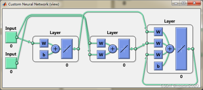
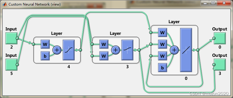
%% 使用view(net)观察神经网络结构。
view(net)
% 此时神经网络有两个输入，三个神经元层。但请注意：net.numInputs设置的是
% 神经网络的输入个数，每个输入的维数是由net.inputs{
    
    i}.size控制。

%%  阈值连接定义
net.biasConnect(1) = 1;
net.biasConnect(3) = 1;
% 或者使用net.biasConnect = [1; 0; 1];
view(net)

%% 输入与层连接定义
net.inputConnect(1,1) = 1;
net.inputConnect(2,1) = 1;
net.inputConnect(2,2) = 1;
% 或者使用net.inputConnect = [1 0; 1 1; 0 0];
view(net)
net.layerConnect = [0 0 0; 0 0 0; 1 1 1];
view(net)
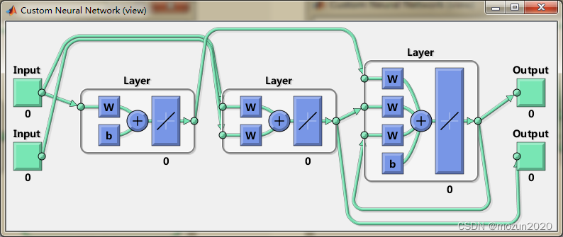
%% 输出连接设置 
net.outputConnect = [0 1 1];
view(net)

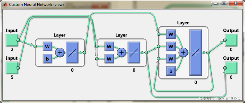
%% 输入设置
net.inputs
net.inputs{
    
    1}
net.inputs{
    
    1}.processFcns = {
    
    'removeconstantrows','mapminmax'};
net.inputs{
    
    2}.size = 5;
net.inputs{
    
    1}.exampleInput = [0 10 5; 0 3 10];
view(net)

%% 层设置
net.layers{
    
    1}
% 将神经网络第一层的神经元个数设置为4个，其传递函数设置为“tansig”并
% 将其初始化函数设置为Nguyen-Widrow函数。
net.layers{
    
    1}.size = 4;
net.layers{
    
    1}.transferFcn = 'tansig';
net.layers{
    
    1}.initFcn = 'initnw';
% 将第二层神经元个数设置为3个，其传递函数设置为“logsig”，并使用“initnw”初始化。
net.layers{
    
    2}.size = 3;
net.layers{
    
    2}.transferFcn = 'logsig';
net.layers{
    
    2}.initFcn = 'initnw';
% 将第三层初始化函数设置为“initnw”
net.layers{
    
    3}.initFcn = 'initnw';
view(net)

%% 输出设置
net.outputs
net.outputs{
    
    2}

%% 阈值，输入权值与层权值设置
net.biases
net.biases{
    
    1}
net.inputWeights
net.layerWeights

%% 将神经网络的某些权值的延迟进行设置 
net.inputWeights{
    
    2,1}.delays = [0 1];
net.inputWeights{
    
    2,2}.delays = 1;
net.layerWeights{
    
    3,3}.delays = 1;

%% 网络函数设置
% 将神经网络初始化设置为“initlay”，这样神经网络就可以按照
% 我们设置的层初始化函数“ initnw”即Nguyen-Widrow进行初始化。
net.initFcn = 'initlay';
% 将神经网络的误差设置为“mse”（mean squared error），同时将神经网络的训练函数
% 设置为“trainlm”Levenberg-Marquardt backpropagation)。
net.performFcn = 'mse';
net.trainFcn = 'trainlm';
% 为了使神经网络可以随机划分训练数据集，我们可以将divideFcn设置为“dividerand”。
net.divideFcn = 'dividerand';
% 将 plot functions设置为：“plotperform”,“plottrainstate”
net.plotFcns = {
    
    'plotperform','plottrainstate'};

%% 权值阈值大小设置
net.IW{
    
    1,1}, net.IW{
    
    2,1}, net.IW{
    
    2,2}
net.LW{
    
    3,1}, net.LW{
    
    3,2}, net.LW{
    
    3,3}
net.b{
    
    1}, net.b{
    
    3}

%% 神经网络初始化
net = init(net);
net.IW{
    
    1,1}

%% 神经网络的训练
X = {
    
    [0; 0] [2; 0.5]; [2; -2; 1; 0; 1] [-1; -1; 1; 0; 1]};
T = {
    
    [1; 1; 1] [0; 0; 0]; 1 -1};
Y = sim(net,X)

%% 神经网络的训练参数
net.trainParam

%%  训练网络
net = train(net,X,T);

%% 仿真来检查神经网络是否相应正常。
Y = sim(net,X)
toc

添加完毕，点击“运行”，开始仿真，输出仿真结果如下：

net =

    Neural Network
 
              name: 'Custom Neural Network'
          userdata: (your custom info)
 
    dimensions:
 
         numInputs: 0
         numLayers: 0
        numOutputs: 0
    numInputDelays: 0
    numLayerDelays: 0
 numFeedbackDelays: 0
 numWeightElements: 0
        sampleTime: 1
 
    connections:
 
       biasConnect: []
      inputConnect: []
      layerConnect: []
     outputConnect: []
 
    subobjects:
 
            inputs: {
    
    0x1 cell array of 0 inputs}
            layers: {
    
    0x1 cell array of 0 layers}
           outputs: {
    
    1x0 cell array of 0 outputs}
            biases: {
    
    0x1 cell array of 0 biases}
      inputWeights: {
    
    0x0 cell array of 0 weights}
      layerWeights: {
    
    0x0 cell array of 0 weights}
 
    functions:
 
          adaptFcn: (none)
        adaptParam: (none)
          derivFcn: 'defaultderiv'
         divideFcn: (none)
       divideParam: (none)
        divideMode: 'sample'
           initFcn: 'initlay'
        performFcn: 'mse'
      performParam: .regularization, .normalization
          plotFcns: {
    
    }
        plotParams: {
    
    1x0 cell array of 0 params}
          trainFcn: (none)
        trainParam: (none)
 
    weight and bias values:
 
                IW: {
    
    0x0 cell} containing 0 input weight matrices
                LW: {
    
    0x0 cell} containing 0 layer weight matrices
                 b: {
    
    0x1 cell} containing 0 bias vectors
 
    methods:
 
             adapt: Learn while in continuous use
         configure: Configure inputs & outputs
            gensim: Generate Simulink model
              init: Initialize weights & biases
           perform: Calculate performance
               sim: Evaluate network outputs given inputs
             train: Train network with examples
              view: View diagram
       unconfigure: Unconfigure inputs & outputs
 

ans = 

    [1x1 nnetInput]
    [1x1 nnetInput]


ans = 

    Neural Network Input

              name: 'Input'
    feedbackOutput: []
       processFcns: {
    
    }
     processParams: {
    
    1x0 cell array of 0 params}
   processSettings: {
    
    0x0 cell array of 0 settings}
    processedRange: []
     processedSize: 0
             range: []
              size: 0
          userdata: (your custom info)


ans = 

    Neural Network Layer
 
              name: 'Layer'
        dimensions: 0
       distanceFcn: (none)
     distanceParam: (none)
         distances: []
           initFcn: 'initwb'
       netInputFcn: 'netsum'
     netInputParam: (none)
         positions: []
             range: []
              size: 0
       topologyFcn: (none)
       transferFcn: 'purelin'
     transferParam: (none)
          userdata: (your custom info)
 

ans = 

    []    [1x1 nnetOutput]    [1x1 nnetOutput]


ans = 

    Neural Network Output

              name: 'Output'
     feedbackInput: []
     feedbackDelay: 0
      feedbackMode: 'none'
       processFcns: {
    
    }
     processParams: {
    
    1x0 cell array of 0 params}
   processSettings: {
    
    0x0 cell array of 0 settings}
    processedRange: [3x2 double]
     processedSize: 3
             range: [3x2 double]
              size: 3
          userdata: (your custom info)


ans = 

    [1x1 nnetBias]
    []
    [1x1 nnetBias]


ans = 

    Neural Network Bias

           initFcn: (none)
             learn: true
          learnFcn: (none)
        learnParam: (none)
              size: 4
          userdata: (your custom info)


ans = 

    [1x1 nnetWeight]                  []
    [1x1 nnetWeight]    [1x1 nnetWeight]
                  []                  []


ans = 

                  []                  []                  []
                  []                  []                  []
    [1x1 nnetWeight]    [1x1 nnetWeight]    [1x1 nnetWeight]


ans =

     0     0
     0     0
     0     0
     0     0


ans =

     0     0     0     0
     0     0     0     0
     0     0     0     0


ans =

     0     0     0     0     0
     0     0     0     0     0
     0     0     0     0     0


ans =

   空矩阵: 0×4


ans =

   空矩阵: 0×3


ans =

     []


ans =

     0
     0
     0
     0


ans =

   空矩阵: 0×1


ans =

    1.9468    2.0124
    2.3881   -1.4619
   -1.7285    2.2028
   -0.2749    2.7865


Y = 

    [3x1 double]    [3x1 double]
    [0x1 double]    [0x1 double]


ans = 

 
    Function Parameters for 'trainlm'
 
    Show Training Window Feedback   showWindow: true
    Show Command Line Feedback showCommandLine: false
    Command Line Frequency                show: 25
    Maximum Epochs                      epochs: 1000
    Maximum Training Time                 time: Inf
    Performance Goal                      goal: 0
    Minimum Gradient                  min_grad: 1e-07
    Maximum Validation Checks         max_fail: 6
    Mu                                      mu: 0.001
    Mu Decrease Ratio                   mu_dec: 0.1
    Mu Increase Ratio                   mu_inc: 10
    Maximum mu                          mu_max: 10000000000
 

Y = 

    [3x1 double]    [3x1 double]
    [    1.0000]    [   -1.0000]

时间已过 3.932652 秒。

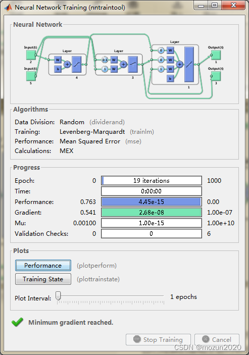
依次点击Plots中的Performance，Training State可得以下图示：

3. 小结

本章介绍了定制神经网络的方法，包括如何设置网络，如何链接网络，并通过对输入输出，连接阈值，输入的连接，输出的连接等进行相应设置，从而得到自己所需的神经网络，再导入数据进行相应的训练，得到模型后再进行预测检验，一个完整的定制神经网络的过程即已实现。对本章内容感兴趣或者想充分学习了解的，建议去研习书中第四十一章节的内容。后期会对其中一些知识点在自己理解的基础上进行补充，欢迎大家一起学习交流。