Machine Learning（7）Neural network —— optimization techniques I

Chenjing Ding
2018/02/27

notation	meaning
g(x)	activate function
$x_n$	the n-th input vector (simplified as $x_i$ when n is not specified)
$x_{n_i}$	the i-th entry of $x_n$ (simplified as $x_i$ when n is not specified)
N	the number of input vectors
K	the number of classes
$t_n$	a vector with K dimensional with k-th entry 1 only when the n-th input vector belongs to k-th class, tn = (0,0,…1…0)
$y_j(x)$	the output of j-th output neural
$y(x)$	a output vector of input vector x; $y(x) = (y_1(x)...y_K(x))$
$W_{ji}^{\tau+1}$	the ( $\tau+1$ )-th update of weight $W_{ji}$
$W_{ji}^{\tau}$	the $\tau$ -th update of weight $W_{ji}$
$\frac{\partial E(W)}{\partial W_{ij}^{(m)}}$	the gradient of m-th layer weight
$l_i$	the number of neural in i-th layer(simplified as l when i is not specified)
$W_{ji}^{(mn)}$	the weight between layer m and n

1. Regularization

To avoid overfitting:

E (W) = \sum_{i = 1}^{n} L (t_{n}, y (x_{n})) + λ Ω (W)

$E(W) = \sum_{i=1}^n L(t_n,y(x_n)) + \lambda \Omega(W)$

L (t_{n}, y (x_{n}))

$L(t_n,y(x_n))$ is a loss function

Ω (W)

$\Omega(W)$ is regularizers：L2 regularizer is

| | W | |^{2} = \sum_{i} \sum_{j} w_{j i}^{2}

$||W||^2 = \sum_i \sum_j w_{ji}^2$ ; L1 regularizer is

| W | = \sum_{i} \sum_{j} | w_{j i} |

$|W| = \sum_i \sum_j |w_{ji}|$ ;

λ

$\lambda$ is regularization parameter;
This means every weight

w_{j i}

$w_{ji}$ can not be too big, thus the model cannot be too complex including so many useless features.

1.what is L1, L2 regularization :
https://www.youtube.com/watch?v=TmzzQoO8mr4 (Chinese)

2.Regularization and Cost Function
https://www.youtube.com/watch?v=KvtGD37Rm5I&list=PLLssT5z_DsK-h9vYZkQkYNWcItqhlRJLN&index=40

2.Normalizing the Inputs

Convergence is faster if:

the mean of all input data is 0
$\frac{ \partial E(W)}{ \partial w_{ji}} = y_i g' \frac{\partial E(W)}{\partial y_j}$ ,weights can only change together if input vector are all positive ao negative, thus it will lead to slow convergence.
the variance of all input data is the same
all input data are not correlated if possible (using PCA to decorrelate them)
if the input are correlated, the direction of steepest descent is not optimal, maybe perpendicular to the direction towards the minimum.

3.Commonly Used Nonlinearities

??????????????The activation function is often nonlinear, here are some.

logistic sigmoid

$σ (a) = \frac{1}{1 + e x p (- a)}; σ^{'} (a) = σ (a) (1 - σ (a));$ $\sigma(a) = \frac{1}{1+exp(-a)}; \\ \sigma'(a) =\sigma(a)(1-\sigma(a));$
tanh

扫描二维码关注公众号，回复： 3817152 查看本文章
$t a n h (a) = 2 σ (2 a) - 1; t a n h^{'} (a) = 1 - t a n h^{2} (a)$ $tanh(a) = 2 \sigma(2a) -1 ;\\tanh'(a) = 1-tanh^2(a)$
Advantages: compared with logistic sigmoid

$tanh(a)$ already centred at zero , thus often converge faster than the standard logistic sigmoid.

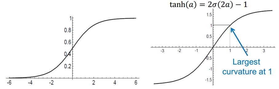
figure1 nonlinear activation function(left: logistic sigmoid; right: tanh)

softmax

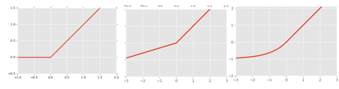
$g_{i} (a) = \frac{e x p (- a_{i})}{\sum_{j} e x p (- a_{j})} s o f t m a x (a + b) = s o f t m a x (a) (b o t h a a n d b a r e v e c t o r s)$ $g_i(a) = \frac{exp(-a_i)}{\sum_j exp(-a_j)}\\ softmax( a + b) = softmax(a) (both\ a\ and\ b\ are \ vectors)$
ReLU

$g (a) = m a x {0, a} g^{'} (a) = {_{0, e l s e}^{1, a > 0}$

Advantages:
1. thus gradient will be passed with a constant factor( $\frac{ \partial E(W)}{ \partial w_{ji}} = y_i g' \frac{\partial E(W)}{\partial y_j}$ ), make it easier to propagate gradient through deep networks.( Imagine $g'<0$ , then $\frac{ \partial E(W)}{ \partial w_{ji}}$ will be smaller and smaller with the networks deep, finally the gradient will be close to zero)
2. don’t need to store ReLU output separately
  Reduction of the required memory by half compared with tanh!
  Because of these two features,ReLU has become the de-facto standard for deep networks.
Disadvantages:
1. stuck at zero, if the output of ReLU is zero for the input vector, then the concerned gradient can not be passed to next layer down since it is zero.
2. Offset bias since it is always positive.
Leaky ReLU

$g (a) = m a x {β a, a}$

Advantages:
1. avoid “stuck at zero”
2. weaker offset bias.
ELU

$g (a) = {_{a, a < 0}^{e^{a} - 1, a >= 0}$ $g(a) = \lbrace_{ \ \ a ,\ \ a<0}^{\ \ e^a-1,\ a >= 0}$
no offset bias but needs to store the activation.

figure2 left:ReLU middle: Leaky ReLU right: ELU
usage of nonlinear function
1. Output nodes
  2 class classfication: sigmoid
  multi-class classification: softmax
  regression tasks: tanh
2. Internal nodes
  tanh is better than sigmoid for internal nodes since it is already centered at 0;

4.Weight Initialization

If we normalize all the input data, we also want to reserve the variance of input data because that the output data which is the input data of next layer again will have the same variance. As a result, convergence will be faster.
Thus our goal is to let variance of input data and output data be same.

y_{j} (x) = \sum_{i = 1}^{l} w_{j i} x_{i} V a r (w_{j i} x_{i}) = E (x_{i})^{2} * V a r (w_{j i}) + E (w_{j i})^{2} * V a r (x_{i}) + V a r (w_{j i}) V a r (x_{i})

$y_j(x) = \sum_{i = 1}^ l w_{ji} x_i\\ Var(w_{ji} x_i) =E(x_i)^2*Var(w_{ji}) + E(w_{ji})^2*Var(x_i) +Var(w_{ji})Var(x_i)$
if the mean of input data and weights are zero and they are identical independent distributed

V a r (w_{j i} x_{i}) = V a r (w_{j i}) V a r (x_{i}) V a r (y_{j} (x)) = \sum_{i = 1}^{l} V a r (w_{j i}) V a r (x_{i}) = l V a r (w_{j i}) V a r (x_{i})

$Var(w_{ji} x_i) = Var(w_{ji})Var(x_i) \\Var(y_j(x) ) = \sum_{i=1}^l Var(w_{ji})Var(x_i)=l Var(w_{ji})Var(x_i)$

4.1 Glorot Initialization

If $Var(w_{ji}) = \frac{1}{l_{in}} \Rightarrow Var(y_j(x)) = Var(x_i)$ ; $l_{in}$ is the number of input neural linked to j-th output neural. If we do the same for the backpropagated gradient ( $l=l_{out}$ ), then $Var(w_{ji}) = \frac{1}{l_{out}}$ .
The glorot initialization is:

V a r (w_{j i}) = \frac{2}{l_{i n} + l_{o u t}}

$Var(w_{ji}) = \frac{2}{l_{in} + l_{out}}$

4.2 He Initialization

The glorot initialization was based on tanh(centred at 0), He et al. made the derivations, proposed to use instead based on ReLU:

V a r (W) = \frac{2}{l_{i n}}

$Var(W) = \frac{2}{l_{in}}$

5.Stochastic and Batch learning

In Gradient Descent, the last step is to adjust weights in the direction of gradients. The equation is:

5.1 Batch learning

Process the full data at once to computer the gradient.

E (W) = \sum_{i = 1}^{N} E_{i} (W) w_{j i}^{τ + 1} = w_{j i}^{τ} - η \frac{\partial E (W)}{\partial W_{j i}^{τ}}

$E(W) = \sum_{i=1}^N E_i(W)\\w_{ji}^{\tau +1} = w_{ji}^{\tau} - \eta \frac{\partial E(W)}{\partial W_{ji}^{\tau}}$

5.2 Stochastic learning

Choose a single training sample $x_n$ to obtain $E_n(W)$ ;

w_{j i}^{τ + 1} = w_{j i}^{τ} - η \frac{\partial E_{n} (W)}{\partial W_{j i}^{τ}}

$w_{ji}^{\tau +1} = w_{ji}^{\tau} - \eta \frac{\partial E_n(W)}{\partial W_{ji}^{\tau}}$

5.3 Stochastic vs. Batch Learning

5.3.1 Batching learning advantages

Many acceleration techniques (e.g., conjugate gradients) only operate in batch learning.
Theoretical analysis of the weight dynamics and convergence rates are simpler.

5.3.2 Stochastic advantages

Usually much faster than batch learning.
Often results in better solutions.
Can be used for tracking changes.

5.4 Minibatch

Minibatch combine two methods above together, process only a small batch of training examples together.

5.4.1 Advantages

more stable than stochastic learning but faster than batch learning
take advantage of redundancies in training data(some training sample can appear in different mini batches)
the input data is matrix since it’s the combination of input vector, and matrix operations is more efficient than vector operations

5.4.2 Caveat

The error function needs to be normalized by minibatch size because we want to keep the learning rate same in different minibatches. Suppose M is the minibatch size:

E (W) = \frac{1}{M} \sum_{i = 1}^{M} E_{i} (W) + \frac{λ}{M} Ω (W)

$E(W) = \frac{1}{M}\sum_{i=1}^M E_i(W) +\frac{\lambda}{M} \Omega(W)$