此处处理非结构化数据(即自然语言)。
1.item_description(描述)
计算描述的字符长度
def wordCount(text):
    # convert to lower case and strip regex
    try:
         # convert to lower case and strip regex
        text = text.lower()
        regex = re.compile('[' +re.escape(string.punctuation) + '0-9\\r\\t\\n]')
        txt = regex.sub(" ", text)
        # tokenize
        # words = nltk.word_tokenize(clean_txt)
        # remove words in stop words
        words = [w for w in txt.split(" ") \
                 if not w in stop_words.ENGLISH_STOP_WORDS and len(w)>3]
        return len(words)
    except:
        return 0

# add a column of word counts to both the training and test set
train['desc_len'] = train['item_description'].apply(lambda x: wordCount(x))
test['desc_len'] = test['item_description'].apply(lambda x: wordCount(x))

train.head()

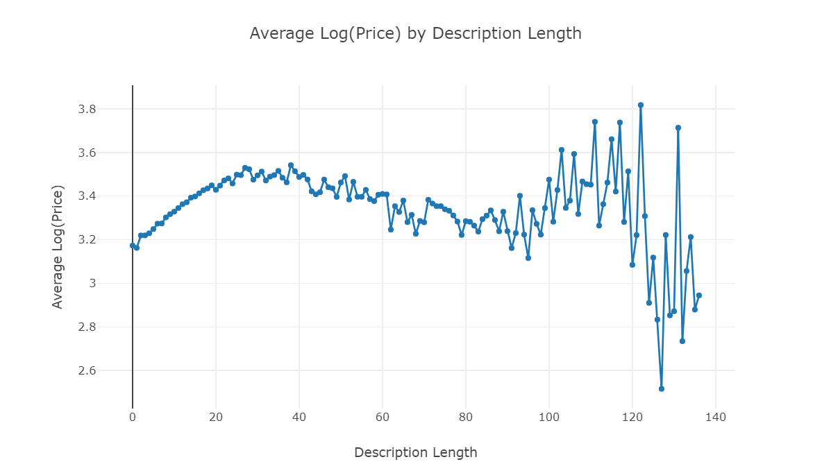
分析价格和字符长度之间的关系
df = train.groupby('desc_len')['price'].mean().reset_index()

trace1 = go.Scatter(
    x = df['desc_len'],
    y = np.log(df['price']+1),
    mode = 'lines+markers',
    name = 'lines+markers'
)
layout = dict(title= 'Average Log(Price) by Description Length',
              yaxis = dict(title='Average Log(Price)'),
              xaxis = dict(title='Description Length'))
fig=dict(data=[trace1], layout=layout)
py.iplot(fig)
移除异常值(即没有描述的行)
预处理:分词
1.先把描述拆分成句子,然后再把句子拆分成单词
扫描二维码关注公众号,回复:
104592 查看本文章

2.移除标点和停词
3.单词小写
4.考虑单词长度等于或者大于3
stop = set(stopwords.words('english'))
def tokenize(text):
    """
    sent_tokenize(): segment text into sentences
    word_tokenize(): break sentences into words
    """
    try:
        regex = re.compile('[' +re.escape(string.punctuation) + '0-9\\r\\t\\n]')
        text = regex.sub(" ", text) # remove punctuation

        tokens_ = [word_tokenize(s) for s in sent_tokenize(text)]
        tokens = []
        for token_by_sent in tokens_:
            tokens += token_by_sent
        tokens = list(filter(lambda t: t.lower() not in stop, tokens))
        filtered_tokens = [w for w in tokens if re.search('[a-zA-Z]', w)]
        filtered_tokens = [w.lower() for w in filtered_tokens if len(w)>=3]

        return filtered_tokens

    except TypeError as e: print(text,e)
# apply the tokenizer into the item descriptipn column
train['tokens'] = train['item_description'].map(tokenize)
test['tokens'] = test['item_description'].map(tokenize)
查看分词效果
for description, tokens in zip(train['item_description'].head(),
                              train['tokens'].head()):
    print('description:', description)
    print('tokens:', tokens)
    print()

使用词云查看描述的词汇在每个标签中出现的频率
# build dictionary with key=category and values as all the descriptions related.
cat_desc = dict()
for cat in general_cats:
    text = " ".join(train.loc[train['general_cat']==cat, 'item_description'].values)
    cat_desc[cat] = tokenize(text)


# find the most common words for the top 4 categories
women100 = Counter(cat_desc['Women']).most_common(100)
beauty100 = Counter(cat_desc['Beauty']).most_common(100)
kids100 = Counter(cat_desc['Kids']).most_common(100)
electronics100 = Counter(cat_desc['Electronics']).most_common(100)
def generate_wordcloud(tup):
    wordcloud = WordCloud(background_color='white',
                          max_words=50, max_font_size=40,
                          random_state=42
                         ).generate(str(tup))
    return wordcloud
fig,axes = plt.subplots(2, 2, figsize=(30, 15))

ax = axes[0, 0]
ax.imshow(generate_wordcloud(women100), interpolation="bilinear")
ax.axis('off')
ax.set_title("Women Top 100", fontsize=30)

ax = axes[0, 1]
ax.imshow(generate_wordcloud(beauty100))
ax.axis('off')
ax.set_title("Beauty Top 100", fontsize=30)

ax = axes[1, 0]
ax.imshow(generate_wordcloud(kids100))
ax.axis('off')
ax.set_title("Kids Top 100", fontsize=30)

ax = axes[1, 1]
ax.imshow(generate_wordcloud(electronics100))
ax.axis('off')
ax.set_title("Electronic Top 100", fontsize=30)

预处理:tf-idf
使用tf-idf计算每个词的在文本中的重要性
from sklearn.feature_extraction.text import TfidfVectorizer
vectorizer = TfidfVectorizer(min_df=10,
                             max_features=180000,
                             tokenizer=tokenize,
                             ngram_range=(1, 2))
all_desc = np.append(train['item_description'].values, test['item_description'].values)
vz = vectorizer.fit_transform(list(all_desc))
vz是一个tfidf矩阵:
·行数是描述的总书
·列数是相应描述在词上的个数
计算tfidf值
#  create a dictionary mapping the tokens to their tfidf values
tfidf = dict(zip(vectorizer.get_feature_names(), vectorizer.idf_))
tfidf = pd.DataFrame(columns=['tfidf']).from_dict(
                    dict(tfidf), orient='index')
tfidf.columns = ['tfidf']
查看tfidf值最小的10个词
tfidf.sort_values(by=['tfidf'], ascending=True).head(10)

查看tfidf值最大的10个词
tfidf.sort_values(by=['tfidf'], ascending=False).head(10)

由于tfidf矩阵太大,我们需要对他进行降维
这里使用t-SNE算法进行降维,但是t-SNE算法的时间复杂度相对较高,tfidf矩阵维度
又太大,我们需要先使用SVD先把矩阵降到50维,然后再使用t-SNE
trn = train.copy()
tst = test.copy()
trn['is_train'] = 1
tst['is_train'] = 0

sample_sz = 15000

combined_df = pd.concat([trn, tst])
combined_sample = combined_df.sample(n=sample_sz)
vz_sample = vectorizer.fit_transform(list(combined_sample['item_description']))
from sklearn.decomposition import TruncatedSVD

n_comp=30
svd = TruncatedSVD(n_components=n_comp, random_state=42)
svd_tfidf = svd.fit_transform(vz_sample)
使用t-SNE
from sklearn.manifold import TSNE
tsne_model = TSNE(n_components=2, verbose=1, random_state=42, n_iter=500)
tsne_tfidf = tsne_model.fit_transform(svd_tfidf)

进行可视化数据
output_notebook()
plot_tfidf = bp.figure(plot_width=700, plot_height=600,
                       title="tf-idf clustering of the item description",
    tools="pan,wheel_zoom,box_zoom,reset,hover,previewsave",
    x_axis_type=None, y_axis_type=None, min_border=1)
combined_sample.reset_index(inplace=True, drop=True)
tfidf_df = pd.DataFrame(tsne_tfidf, columns=['x', 'y'])
tfidf_df['description'] = combined_sample['item_description']
tfidf_df['tokens'] = combined_sample['tokens']
tfidf_df['category'] = combined_sample['general_cat']
plot_tfidf.scatter(x='x', y='y', source=tfidf_df, alpha=0.7)
hover = plot_tfidf.select(dict(type=HoverTool))
hover.tooltips={"description": "@description", "tokens": "@tokens", "category":"@category"}
show(plot_tfidf)

图中颜色深的圆点是因为数量多导致的
2.使用k-means进行聚类
from sklearn.cluster import MiniBatchKMeans

num_clusters = 30 # need to be selected wisely
kmeans_model = MiniBatchKMeans(n_clusters=num_clusters,
                               init='k-means++',
                               n_init=1,
                               init_size=1000, batch_size=1000, verbose=0, max_iter=1000)
kmeans = kmeans_model.fit(vz)
kmeans_clusters = kmeans.predict(vz)
kmeans_distances = kmeans.transform(vz)
sorted_centroids = kmeans.cluster_centers_.argsort()[:, ::-1]
terms = vectorizer.get_feature_names()

for i in range(num_clusters):
    print("Cluster %d:" % i)
    aux = ''
    for j in sorted_centroids[i, :10]:
        aux += terms[j] + ' | '
    print(aux)
    print()
聚类完成后 我们需要把他降到二维来展示
# repeat the same steps for the sample
kmeans = kmeans_model.fit(vz_sample)
kmeans_clusters = kmeans.predict(vz_sample)
kmeans_distances = kmeans.transform(vz_sample)
# reduce dimension to 2 using tsne
tsne_kmeans = tsne_model.fit_transform(kmeans_distances)
#combined_sample.reset_index(drop=True, inplace=True)
kmeans_df = pd.DataFrame(tsne_kmeans, columns=['x', 'y'])
kmeans_df['cluster'] = kmeans_clusters
kmeans_df['description'] = combined_sample['item_description']
kmeans_df['category'] = combined_sample['general_cat']
#kmeans_df['cluster']=kmeans_df.cluster.astype(str).astype('category')
plot_kmeans = bp.figure(plot_width=700, plot_height=600,
                        title="KMeans clustering of the description",
    tools="pan,wheel_zoom,box_zoom,reset,hover,previewsave",
    x_axis_type=None, y_axis_type=None, min_border=1)
source = ColumnDataSource(data=dict(x=kmeans_df['x'], y=kmeans_df['y'],
                                    color=colormap[kmeans_clusters],
                                    description=kmeans_df['description'],
                                    category=kmeans_df['category'],
                                    cluster=kmeans_df['cluster']))

plot_kmeans.scatter(x='x', y='y', color='color', source=source)
hover = plot_kmeans.select(dict(type=HoverTool))
hover.tooltips={"description": "@description", "category": "@category", "cluster":"@cluster" }
show(plot_kmeans)

使用LDA进行文本主题提取
它的输入是一个词库,即每个文档表示为一行,每列包含语料库中单词的计数。
我们将使用一个称为pyLDAvis的强大工具,为我们提供LDA的交互式可视化。
cvectorizer = CountVectorizer(min_df=4,
                              max_features=180000,
                              tokenizer=tokenize,
                              ngram_range=(1,2))
cvz = cvectorizer.fit_transform(combined_sample['item_description'])
lda_model = LatentDirichletAllocation(n_components=20,
                                      learning_method='online',
                                      max_iter=20,
                                      random_state=42)
X_topics = lda_model.fit_transform(cvz)
n_top_words = 10
topic_summaries = []

topic_word = lda_model.components_  # get the topic words
vocab = cvectorizer.get_feature_names()

for i, topic_dist in enumerate(topic_word):
    topic_words = np.array(vocab)[np.argsort(topic_dist)][:-(n_top_words+1):-1]
    topic_summaries.append(' '.join(topic_words))
    print('Topic {}: {}'.format(i, ' | '.join(topic_words)))

降维
# reduce dimension to 2 using tsne
tsne_lda = tsne_model.fit_transform(X_topics)

unnormalized = np.matrix(X_topics)
doc_topic = unnormalized/unnormalized.sum(axis=1)

lda_keys = []
for i, tweet in enumerate(combined_sample['item_description']):
    lda_keys += [doc_topic[i].argmax()]

lda_df = pd.DataFrame(tsne_lda, columns=['x','y'])
lda_df['description'] = combined_sample['item_description']
lda_df['category'] = combined_sample['general_cat']
lda_df['topic'] = lda_keys
lda_df['topic'] = lda_df['topic'].map(int)
source = ColumnDataSource(data=dict(x=lda_df['x'], y=lda_df['y'],
                                    color=colormap[lda_keys],
                                    description=lda_df['description'],
                                    topic=lda_df['topic'],
                                    category=lda_df['category']))

plot_lda.scatter(source=source, x='x', y='y', color='color')
hover = plot_kmeans.select(dict(type=HoverTool))
hover = plot_lda.select(dict(type=HoverTool))
hover.tooltips={"description":"@description",
                "topic":"@topic", "category":"@category"}
show(plot_lda)

def prepareLDAData():
    data = {
        'vocab': vocab,
        'doc_topic_dists': doc_topic,
        'doc_lengths': list(lda_df['len_docs']),
        'term_frequency':cvectorizer.vocabulary_,
        'topic_term_dists': lda_model.components_
    }
    return data

import pyLDAvis

lda_df['len_docs'] = combined_sample['tokens'].map(len)
ldadata = prepareLDAData()
pyLDAvis.enable_notebook()
prepared_data = pyLDAvis.prepare(**ldadata)
import IPython.display
from IPython.core.display import display, HTML, Javascript

#h = IPython.display.display(HTML(html_string))
#IPython.display.display_HTML(h)