此代码编写依据 DataCamp 发表的一篇针对 TensorFlow 初学者的教程。此教程从向量和张量的基本概念说起,一步步实现了一个分类交通标志图像的神经网络。
1.加载并预处理数据
数据下载地址:http://btsd.ethz.ch/shareddata/。下载 BelgiumTSC_Training 和 BelgiumTSC_Testing。
数据下载完毕后,提取文件夹,整理好数据存放地址。我的Training和Testing数据存放地址如下:
/home/zhangxueying/images/TrafficSigns/Training
/home/zhangxueying/images/TrafficSigns/Testing
开始导入数据:(并将图片数据信息统一为28x28的灰度图片)
#load data

import os                    #python中的os模块用于处理文件和目录
import skimage               #python中的skimage模块用于图像处理
import numpy as np           #python中的numpy模块用于科学计算
from skimage import data,transform
from skimage.color import rgb2gray     #rgb2gray将图片转化为灰度


#here data_directory="/home/zhangxueying/image/TrafficSigns/Training"
def load_data(data_directory):
    directories=[d for d in os.listdir(data_directory) if os.path.isdir(os.path.join(data_directory,d))]
    #d is every classification file
    labels=[]
    images=[]
    for d in directories:
        #每一类的路径
        label_directory=os.path.join(data_directory,d)
        file_names=[os.path.join(label_directory,f) for f in os.listdir(label_directory) if f.endswith(".ppm")]
        #file_names is every photo which is end with ".ppm"
        for f in file_names:
            images.append(skimage.data.imread(f))   #read image
            labels.append(int(d))                   #read label
    return images,labels

#images and labels are list

ROOT_PATH="/home/zhangxueying/image"
train_data_directory=os.path.join(ROOT_PATH,"TrafficSigns/Training")
test_data_directory=os.path.join(ROOT_PATH,"TrafficSigns/Testing")
images,labels=load_data(train_data_directory)

# Rescale the images in the `images` array
images28 = [transform.resize(image, (28, 28)) for image in images]
# Convert `images28` to an array
images28 = np.array(images28)
# Convert `images28` to grayscale
images28 = rgb2gray(images28)
2.可视化图像
(1)加载和预处理完图像信息后,需要可视化下图像,来判断上述工作的正确性
import matplotlib.pyplot as plt      #python中强大的画图模块
from load import*                    #导入和预处理代码写于load.py中,需要用到其中加载和处理后的images28

traffic_signs = [300, 2250, 3650, 4000]      #随机选取

for i in range(len(traffic_signs)):     #i from 0 to 3
    plt.subplot(1, 4, i + 1)
    plt.axis('off')
    plt.imshow(images28[traffic_signs[i]], cmap="gray")
    #你确实必须指定颜色图(即 cmap),并将其设置为 gray 以给出灰度图像的图表。
    # 这是因为 imshow() 默认使用一种类似热力图的颜色图。
    plt.subplots_adjust(wspace=0.5)       #调整各个图之间的间距

# Show the plot
plt.show()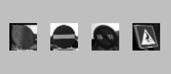
(2)绘制所有 62 个类的整体情况
# Import the `pyplot` module as `plt`
import matplotlib.pyplot as plt
from load import*

# Get the unique labels
unique_labels = set(labels)

# Initialize the figure
plt.figure(figsize=(15, 15))

# Set a counter
i = 1

# For each unique label,
for label in unique_labels:
    # You pick the first image for each label
    image = images28[labels.index(label)]
    # Define 64 subplots
    plt.subplot(8, 8, i)

    # Don't include axes
    plt.axis('off')

    # Add a title to each subplot
    plt.title("Label {0} ({1})".format(label, labels.count(label)))

    # Add 1 to the counter
    i += 1

    # And you plot this first image
    plt.imshow(image)

# Show the plot
plt.show()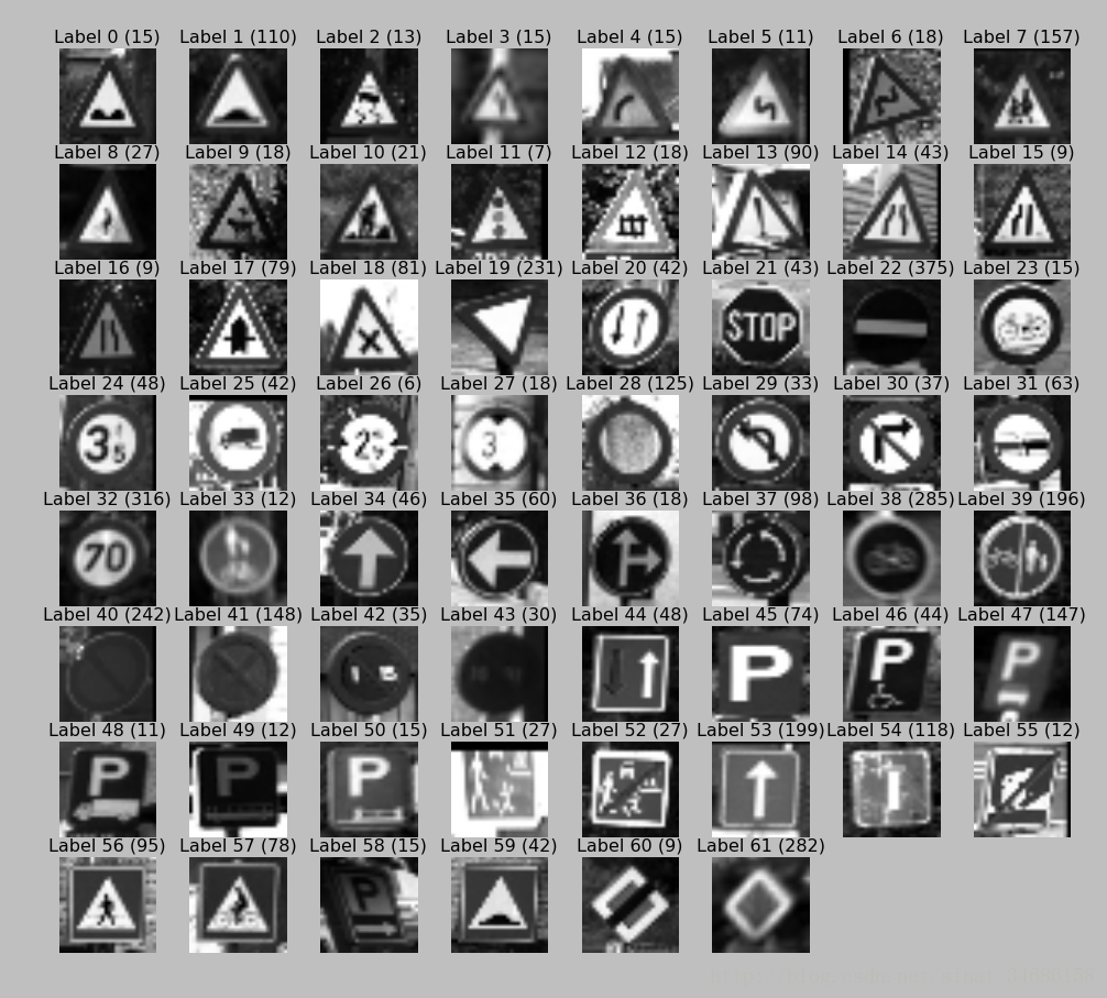
3.训练神经网络
这里使用了全连接神经网络
# Import `tensorflow`
import tensorflow as tf
from load import*

# Initialize placeholders
x = tf.placeholder(dtype=tf.float32, shape=[None, 28, 28])
y = tf.placeholder(tf.int32, [None])


#然后构建你的网络。首先使用 flatten() 函数展平输入,
# 其会给你一个形状为 [None, 784] 的数组,而不是 [None, 28, 28]——这是你的灰度图像的形状。
# Flatten the input data
images_flat = tf.contrib.layers.flatten(x)

# Fully connected layer构建一个全连接层,其可以生成大小为 [None, 62] 的 logits。logits 是运行在早期层未缩放的输出上的函数,其使用相对比例来了解单位是否是线性的。
logits = tf.contrib.layers.fully_connected(images_flat, 62, tf.nn.relu)

# Define a loss function
#定义损失函数了。sparse_softmax_cross_entropy_with_logits(),其可以计算 logits 和标签之间的稀疏 softmax 交叉熵。回归(regression)被用于预测连续值,而分类(classification)则被用于预测离散值或数据点的类别。你可以使用 reduce_mean() 来包裹这个函数,它可以计算一个张量的维度上各个元素的均值。
loss = tf.reduce_mean(tf.nn.sparse_softmax_cross_entropy_with_logits(labels=y,
                                                                     logits=logits))
# Define an optimizer
train_op = tf.train.AdamOptimizer(learning_rate=0.001).minimize(loss)

# Convert logits to label indexes
correct_pred = tf.argmax(logits, 1)

# Define an accuracy metric
accuracy = tf.reduce_mean(tf.cast(correct_pred, tf.float32))

'''print("images_flat: ", images_flat)

print("logits: ", logits)

print("loss: ", loss)

print("predicted_labels: ", correct_pred)
'''
tf.set_random_seed(1234)
sess = tf.Session()

sess.run(tf.global_variables_initializer())

for i in range(201):
    print('EPOCH', i)
    _, accuracy_val = sess.run([train_op, accuracy], feed_dict={x: images28, y: labels})
    if i % 10 == 0:
        print("Loss: ", loss)
    print('DONE WITH EPOCH')
4.评估神经网络
(1)随机选择几张图来大致判断分类的准确性
# Import `matplotlib`
import matplotlib.pyplot as plt
import random       #随机
from nnet import*
# Pick 10 random images
sample_indexes = random.sample(range(len(images28)), 10)
sample_images = [images28[i] for i in sample_indexes]
sample_labels = [labels[i] for i in sample_indexes]

# Run the "correct_pred" operation
predicted = sess.run([correct_pred], feed_dict={x: sample_images})[0]

# Print the real and predicted labels
print(sample_labels)
print(predicted)

# Display the predictions and the ground truth visually.
fig = plt.figure(figsize=(10, 10))
for i in range(len(sample_images)):
    truth = sample_labels[i]
    prediction = predicted[i]
    plt.subplot(5, 2, 1 + i)
    plt.axis('off')
    color = 'green' if truth == prediction else 'red'
    plt.text(40, 10, "Truth:        {0}\nPrediction: {1}".format(truth, prediction),
             fontsize=12, color=color)
    plt.imshow(sample_images[i], cmap="gray")

plt.show()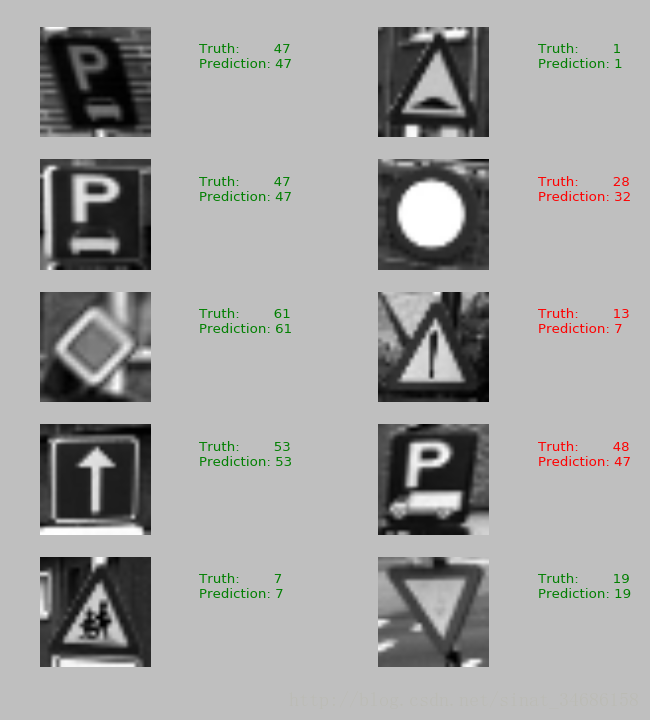
分析图像可知,预测正确的图像有7个,错误的有3个。准确率大致为70%
(2)将建好的模型用测试集数据,来计算准确率
# Import `skimage`
from skimage import transform
from nnet import*

# Load the test data
test_images, test_labels = load_data(test_data_directory)

# Transform the images to 28 by 28 pixels
test_images28 = [transform.resize(image, (28, 28)) for image in test_images]

# Convert to grayscale
from skimage.color import rgb2gray

test_images28 = rgb2gray(np.array(test_images28))

# Run predictions against the full test set.
predicted = sess.run([correct_pred], feed_dict={x: test_images28})[0]

# Calculate correct matches
match_count = sum([int(y == y_) for y, y_ in zip(test_labels, predicted)])

# Calculate the accuracy
accuracy = match_count / len(test_labels)

# Print the accuracy
print("Accuracy: {:.3f}".format(accuracy))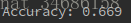
此分类问题比较简单,数据量也较少。
