datawhale第三次打卡

话不多说，直接导入代码和相关文档说明：

import warnings
warnings.filterwarnings('ignore')
import pandas as pd
import numpy as np
import matplotlib.pyplot as plt
import seaborn as sns
import missingno as msno
%matplotlib inline

Train_data = pd.read_csv('used_car_train_20200313.csv', sep=' ')#导入训练集
Test_data = pd.read_csv('used_car_testA_20200313.csv', sep=' ')#导入测试集

def outliers_proc(data,col_name,scale=3):
    '''
    用于清洗数据
    :param data : pandas格式数据
    :col_name : pandas 列名
    :scale : 尺度
    return 异常值删除后的data
    '''
    def box_plot_outliers(data_ser,box_scale):
        '''
        利用箱线图去除异常值
        :data_ser : pandas.Series格式
        :box_scale : 尺度
        '''
        iqr=box_scale*(data_ser.quantile(0.75)-data_ser.quantile(0.25))
        val_low=data_ser.quantile(0.25)-iqr
        val_up=data_ser.quantile(0.75)+iqr
        rule_low=(data_ser<val_low)
        rule_up=(data_ser>val_up)
        return (rule_low,rule_up),(val_low,val_up)
    
    data_n=data.copy()
    data_series=data_n[col_name]
    #删除规则
    rule,value=box_plot_outliers(data_series,box_scale=scale)
    index=np.arange(data_series.shape[0])[rule[0] | rule[1]]
    print("delete num of number is:{}".format(len(index)))
    #删除异常数据
    data_n=data_n.drop(index)
    data_n.reset_index(drop=True,inplace=True)
    print("remaining number is:{}".format(data_n.shape[0]))
    #可视化异常数据对比
    index_low=np.arange(data_series.shape[0])[rule[0]]
    outliers=data_series.iloc[index_low]
    print("the describe of lower is:")
    print(pd.Series(outliers).describe())
    index_up=np.arange(data_series.shape[0])[rule[1]]
    outliers=data_series.iloc[index_up]
    print("the describe of larger is:")
    print(pd.Series(outliers).describe())
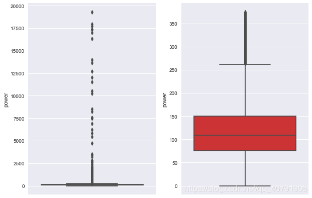
    #箱线图可视化
    fig,ax=plt.subplots(1,2,figsize=(10,7))
    sns.boxplot(y=data[col_name],data=data,palette='Set1',ax=ax[0])
    sns.boxplot(y=data_n[col_name],data=data_n,palette='Set1',ax=ax[1])
    return data_n

dataTrain=outliers_proc(Train_data,'power',3)
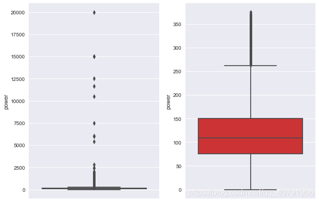
dataTest=outliers_proc(Test_data,'power',3)

delete num of number is:963
remaining number is:149037
the describe of lower is:
count    0.0
mean     NaN
std      NaN
min      NaN
25%      NaN
50%      NaN
75%      NaN
max      NaN
Name: power, dtype: float64
the describe of larger is:
count      963.000000
mean       846.836968
std       1929.418081
min        376.000000
25%        400.000000
50%        436.000000
75%        514.000000
max      19312.000000
Name: power, dtype: float64
delete num of number is:323
remaining number is:49677
the describe of lower is:
count    0.0
mean     NaN
std      NaN
min      NaN
25%      NaN
50%      NaN
75%      NaN
max      NaN
Name: power, dtype: float64
the describe of larger is:
count      323.000000
mean       919.882353
std       2009.860942
min        379.000000
25%        404.000000
50%        450.000000
75%        558.500000
max      20000.000000
Name: power, dtype: float64

#合并训练集和测试集
dataTrain['train']=1
dataTest['train']=0
data=pd.concat([dataTrain,dataTest],ignore_index=True,sort=False)

#使用时间数据来做特征，时间与价格成反比
data['used_time'] = (pd.to_datetime(data['creatDate'],
                            format='%Y%m%d', errors='coerce') -pd.to_datetime(data['regDate'], 
                           format='%Y%m%d', errors='coerce')).dt.days

print("缺失个数：",data['used_time'].isnull().sum())
#有15072个确实值
print("总个数:",len(data))
print('有%.2f%%数据缺失'%(data['used_time'].isnull().sum()/len(data)*100))

#从邮编中获取城市信息，德国
data['city']=data['regionCode'].apply(lambda x:str(x)[:-3])
# print(data['city'])

#计算某品牌的销售统计量

train_gb = dataTrain.groupby('brand')
all_info = {}
for kind, kind_data in train_gb:
    info = {}
    kind_data = kind_data[kind_data['price'] > 0]
    info['brand_amount'] = len(kind_data)
    info['brand_price_max'] = kind_data.price.max()
    info['brand_price_median'] = kind_data.price.median()
    info['brand_price_min'] = kind_data.price.min()
    info['brand_price_sum'] = kind_data.price.sum()
    info['brand_price_std'] = kind_data.price.std()
    info['brand_price_average'] = round(kind_data.price.sum() / (len(kind_data) + 1), 2)
    all_info[kind] = info
brand_fe = pd.DataFrame(all_info).T.reset_index().rename(columns={'index':'brand'})
data = data.merge(brand_fe, how='left', on='brand')

#数据分桶
#离散后稀疏向量内积乘法运算速度更快，计算结果页方便存储，容易扩展
#离散后的特征对异常值更具鲁棒性，如age>30为1否则为0，对于年龄为200的也不会对魔性造成很大的干扰
#LR属于广义线性模型，表达能力有限，经过离散化后，每个变量有单独的权重，这相当于引入了非线性，能够提升模型的表达能力，加大拟合
#离散后特征可以进行特征交叉，提升表达能力，由M+N个变量变成M*N个变量，进一步引入非线性，提升表达能力
#特征离散后模型更稳定，如用户年龄区间不会因为用户增长了一岁就变化
#其他原因，例如LightGBM在改进XGBoost时就增加了数据分桶，增强了模型的泛化性

#以power为例
bin=[i*10 for i in range(31)]
data['power_bin']=pd.cut(data['power'],bin,labels=False)
data[['power_bin','power']].head()

#删除原始数据
data=data.drop(['creatDate','regDate','regionCode'],axis=1)

#导出数据，给树模型使用
data.to_csv('data_for_tree.csv',index=0)

缺失个数： 15057
总个数: 198714
有7.58%数据缺失

#构造LR 数据特征
#不同的模型需要不同的特征
data['power'].plot.hist()
#test数据集中没有做异常值处理
dataTrain['power'].plot.hist()
#对其去log，再归一化
from sklearn import preprocessing
min_max_scaler=preprocessing.MinMaxScaler()
data['power']=np.log(data['power']+1)
data['power']=((data['power'])-np.min(data['power']))/(np.max(data['power'])-np.min(data['power']))
data['power'].plot.hist()

data['kilometer'].plot.hist()

#归一化
data['kilometer']=((data['kilometer']-np.min(data['kilometer']))/
                  np.max(data['kilometer'])-np.min(data['kilometer']))
data['kilometer'].plot.hist()

#对其他特征做归一化
def max_min(x): 
    return (x - np.min(x)) / (np.max(x) - np.min(x))

data['brand_amount'] = max_min(data['brand_amount'])
data['brand_price_average'] = max_min(data['brand_price_average'])
data['brand_price_max'] = max_min(data['brand_price_max'])
data['brand_price_median'] = max_min(data['brand_price_median'])
data['brand_price_min'] = max_min(data['brand_price_min'])
data['brand_price_std'] = max_min(data['brand_price_std'])
data['brand_price_sum'] = max_min(data['brand_price_sum'])

#对类别特征进行one-hot编码
data=pd.get_dummies(data,columns=['model','brand','bodyType','fuelType','gearbox','notRepairedDamage','power_bin'])

#导出数据，给lr模型使用
data.to_csv('data_for_lr.csv',index=0)

#特征筛选
#过滤式
#相关性分析
print(data['power'].corr(data['price'],method='spearman'))
print(data['kilometer'].corr(data['price'],method='spearman'))
print(data['brand_amount'].corr(data['price'],method='spearman'))
print(data['brand_price_average'].corr(data['price'],method='spearman'))
print(data['brand_price_max'].corr(data['price'],method='spearman'))
print(data['brand_price_median'].corr(data['price'],method='spearman'))

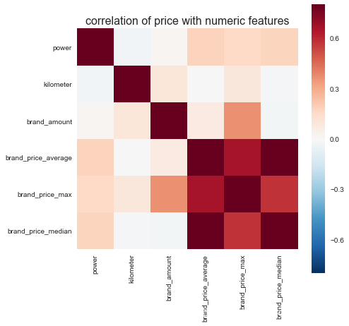
#可视化相关性
data_numeric=data[['power','kilometer','brand_amount','brand_price_average',
                   'brand_price_max','brand_price_median']]
correlation=data_numeric.corr()

f,ax=plt.subplots(figsize=(7,7))
plt.title("correlation of price with numeric features",y=1,size=16)
sns.heatmap(correlation,square=True,vmax=0.8)

0.5728285196051496
-0.4082569701616764
0.058156610025581514
0.3834909576057687
0.259066833880992
0.38691042393409447





<matplotlib.axes._subplots.AxesSubplot at 0x26ef19bca90>

**

总结：
1.特征工程的主要目的还是在于将数据转换为能更好地表示潜在问题的特征，从而提高机器学习的性能，特征构造也属于特征工程的一部分，其目的是为了增强数据的表达，因此特征工程也是和学习模型直接相关的。
2.有些比赛的特征是匿名特征，这导致我们并不清楚特征相互直接的关联性，这时我们就只有单纯基于特征进行处 理，比如装箱，groupby，agg 等这样一些操作进行一些特征统计。
3.此外还可以对特征进行进一步的 log，exp 等 变换，或者对多个特征进行四则运算(例如我们可以通过减法算出使用时长)，多项式组合等然后进行筛选。由于特性的 匿名性其实限制了很多对于特征的处理，当然有些时候用 NN 去提取一些特征也会达到意想不到的良好效果。

**