机器学习算法练习之（一）：Python实现logistic回归

第一步：生成数据并可视化

import numpy as np
import matplotlib.pyplot as plt

np.random.seed(12)
num_observations=5000
#生成二维高斯分布数据
x1 = np.random.multivariate_normal([0, 0], [[1, .75],[.75, 1]], num_observations)
x2 = np.random.multivariate_normal([1, 4], [[1, .75],[.75, 1]], num_observations)

simulated_separableish_features = np.vstack((x1, x2)).astype(np.float32)
simulated_labels = np.hstack((np.zeros(num_observations),
                              np.ones(num_observations)))

plt.figure(figsize=(12,8))
plt.scatter(simulated_separableish_features[:, 0], simulated_separableish_features[:, 1],
            c = simulated_labels, alpha = .4)

plt.figure(figsize=(12,8))
plt.scatter(simulated_separableish_features[:, 0], simulated_separableish_features[:, 1],
            c = simulated_labels, alpha = .4)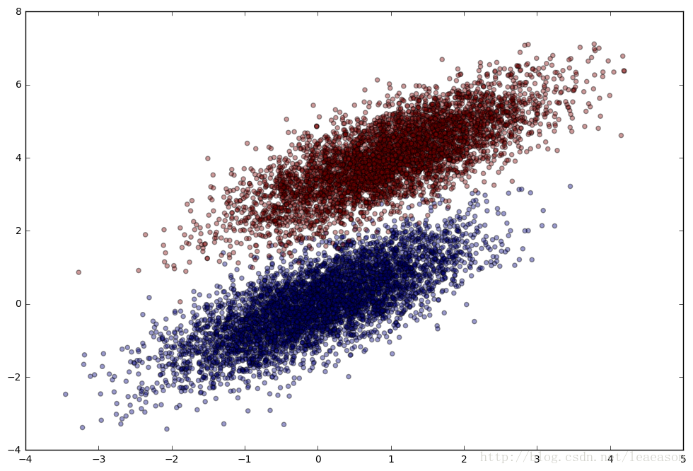

第二步：定义sigmoid函数以及对数似然函数

#定义sigmoid函数
def sigmoid(scores):
    return 1 / (1 + np.exp(-scores))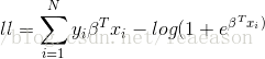

#对数似然估计
def log_likelihood(features, target, weights):
    scores = np.dot(features, weights)
    ll = np.sum( target*scores - np.log(1 + np.exp(scores)) )
    return ll

第三步：定义对数似然回归

#对数似然回归
def logistic_regression(features, target, num_steps, learning_rate, add_intercept = False):
    if add_intercept:
        intercept = np.ones((features.shape[0], 1))
        features = np.hstack((intercept, features))

    weights = np.zeros(features.shape[1])

    for step in range(num_steps):
        scores = np.dot(features, weights)
        predictions = sigmoid(scores)

        # Update weights with gradient
        output_error_signal = target - predictions
        gradient = np.dot(features.T, output_error_signal)
        weights += learning_rate * gradient

        # Print log-likelihood every so often
        if step % 10000 == 0:
            print (log_likelihood(features, target, weights))

    return weights

weights = logistic_regression(simulated_separableish_features, simulated_labels,
                     num_steps = 300000, learning_rate = 5e-5, add_intercept=True)

weights：-4346.26477915
[…]
-140.725421362
-140.725421357
-140.725421355

从sklearn包导入LogisticRegression,得到权值

from sklearn.linear_model import LogisticRegression

clf = LogisticRegression(fit_intercept=True, C = 1e15)
clf.fit(simulated_separableish_features, simulated_labels)

print (clf.intercept_, clf.coef_)
print (weights)

[-13.99400797] [[-5.02712572 8.23286799]]
[-14.09225541 -5.05899648 8.28955762]
第四步：与sklearn得到的训练准确率相比较

data_with_intercept = np.hstack((np.ones((simulated_separableish_features.shape[0], 1)),
                                 simulated_separableish_features))
final_scores = np.dot(data_with_intercept, weights)
preds = np.round(sigmoid(final_scores))

print ('Accuracy from scratch: {0}'.format((preds == simulated_labels).sum().astype(float) / len(preds)))
print ('Accuracy from sk-learn: {0}'.format(clf.score(simulated_separableish_features, simulated_labels)))

Accuracy from scratch: 0.9948
Accuracy from sk-learn: 0.9948

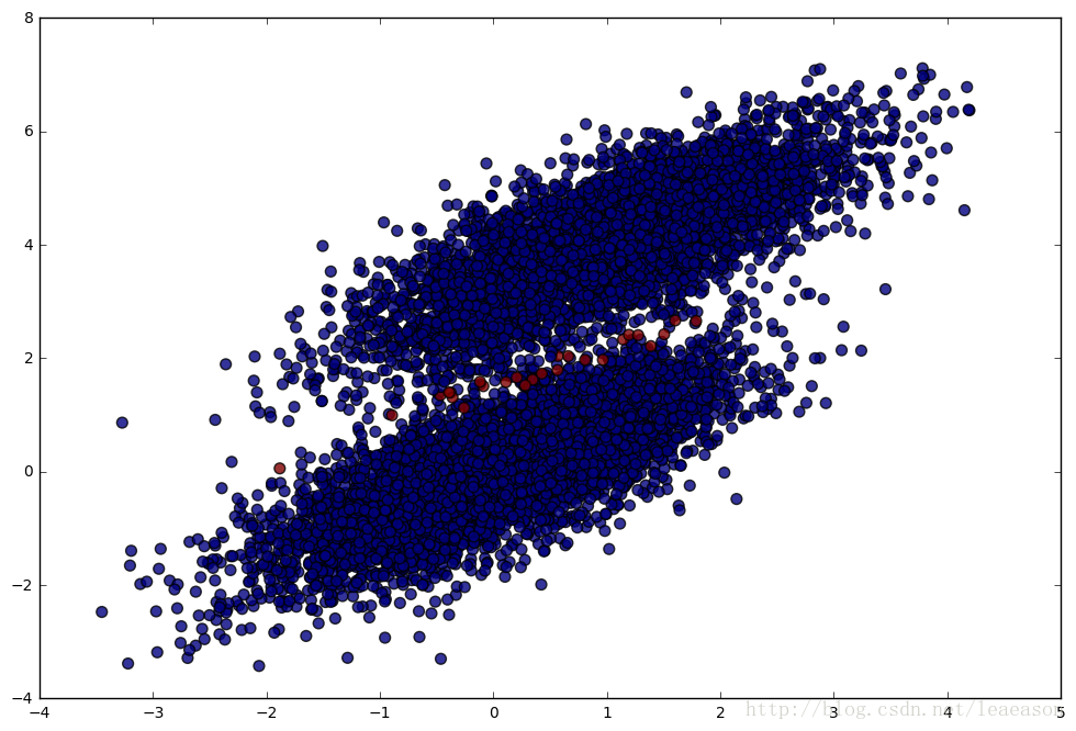
plt.figure(figsize = (12, 8))
plt.scatter(simulated_separableish_features[:, 0], simulated_separableish_features[:, 1],
            c = preds == simulated_labels - 1, alpha = .8, s = 50)

蓝色代表预测正确的数据，红色代表预测错误的数据