Octave Tuturial: Vectorization

摘要: 本文是吴恩达 (Andrew Ng)老师《机器学习》课程，第六章《Octave教程》中第43课时《矢量化》的视频原文字幕。为本人在视频学习过程中记录下来并加以修正，使其更加简洁，方便阅读，以便日后查阅使用。现分享给大家。如有错误，欢迎大家批评指正，在此表示诚挚地感谢！同时希望对大家的学习能有所帮助。

In this video/article, I'd like to tell you the idea of vectorization. So, whether you're using Octave, or a similar language like MATLAT, or whether you're using Python NumPy or Java or C, C++, all of these languages have either built into them or have readily and easily accessible different numerical linear algebra librarilies. They're usually very well written, highly optimized, often developed by people that, you know, have PhDs in numerical computing, or they are really specializing numerical computing. And when you are implementing machine learning algorithms, if you're able to take advantage of these linear algebra librarilies or these numerical linear algebra librariles, and mix the routine calls to them, rather than sort of write call yourself to do things that these librarilies could be doing. If you do that, then often you get code that "first is more efficient". So, just run more quickly and take better advantage of any parallel hardware your computer may have and so on. And second, it also means that you end up with less code that you need to write. So have a simpler implementation. That is, therefore, maybe also more likely to be bug free. And as a concrete example. Rather than writing code yourself to multiply matrices, if you let Octave do it by typing $a\times b$ , that will use a very efficient routine to multiply the 2 matrices. And there's a bunch of examples like these where if you use appropriate vectorized implementations, you get much simpler code, and much more efficient code. Let's look at some examples.

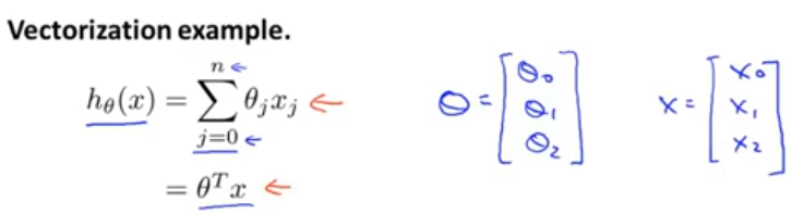
Here's a usual hypothesis of linear regression. And if you want to compute $h_{\theta }(x)$ , notice that there is a sum on the right. And so one thing you could do is compute the sum from $j=0$ to $j=n$ yourself. Another way to think of this is to think of $h_{\theta }(x)=\theta ^{T}x$ . And what you can do is think of this as you know, computing this in a product between 2 vectors, where $\theta=\begin{bmatrix} \theta _{0}\\ \theta _{1}\\ \theta _{2}\\ \end{bmatrix}$ if n=2. And if you think of $x=\begin{bmatrix} x_0\\ x_1\\ x_2 \end{bmatrix}$ . And these 2 views can give you 2 different implementations. Here's what I mean.

Here's an unvectorized implementation for how to compute $h_{\theta}(x)$ . And by unvectorized I mean without vectorization. We might first initialize prediction to be 0.0. This prediction is going to eventually be $h_{\theta}(x)$ . And then I'm going to have a for loop for $j$ equals to 1 through n+1, prediction gets incremented by $\theta(j) \times x(j)$ . So, it's kind of this expression over here. By the way, I should mention in these vectors right over here, I had these vectors being 0-indexed. But because MATLAT is one-indexed, $\theta_0$ in MATLAT, we might end up representing as $\theta_1$ etc. Just because vectors in MATLAT are indexed starting from 1, even though our real $\theta$ and x here indexing from 0. But so, this is an unvectorized implementation in that we have a for loop that you know suming up the n elements of the sum.

In contrast, here's how you write a vectorized implementation. You would think x and $\theta$ as vectors. You just set $prediction=\theta ^{T}x$ . So you instead of writing all these lines of code with the for loop, you instead just have one line of code and what this line of code will do is it uses Octave's highly optimized numerical linear algebra routines to compute this inner product between the two vectors. Not only is the vectorized implementation simpler, it will also run much more efficiently.

So, that was Octave. But issue of vectorization applies to other programming language as well. Let's look at an example in C++.

Here's what an unvectorized implementation might look like. We again initialize $prediction=0.0$ . And then we now have a for loop for j equals 0 up to n.

In contrast, using a good numerical linear algebra library in C++, you can instead write code that might look like this. So, depending on the details of your numerical linear algebra library, you might have an object that is a C++ object which is vector theta, and a C++ object which is a vector x, and you just take $theta.transpose()\times x$ , where this times becomes C++ overload operator. So that you can just multiply these two vectors in C++. And depending on the details of your numerical linear algebra library, you might end up using a slightly different syntax, but by relying on a library to do this in a product, you can get a much simpler piece of code and a much more efficient one.

Let's now look at a more sophisticated example. Just to remind you here's our update rule for gradient descent for linear regression. So we update $\theta _{j}$ using this rule for all values of $j=0,1,2..n$ . And if I just write out these equations for $\theta _{0},\theta _{1},\theta _{2}$ . Assuming we have two features. Then these are updates we perform to $\theta _{0},\theta _{1},\theta _{2}$ . Where you might remember my saying in an earlier video, that these should be simultaneous updates. So, let's see if we can come up with a vectorized implementation of this.

Here are my same 3 equations written on a slightly smaller font, and you can image that one way of implement this three lines of code is have a for loop that says for $j=0,1,2$ , to update $\theta _{j}$ or something like that. But instead, let's come up with a vectorized implementation, and see if we can have a simpler way. So, basically compress these three lines of code or a for loop effectively does these 3 steps 1 step at a time. Let's see how we can take these 3 steps and compress them into 1 line of vectorized code. Here's the idea. What I'm going to do is I'm going to think of $\theta$ as a vector, and I'm going to update $\theta$ as $\theta$ minus $\alpha$ times some other vector, $\delta$ . Where $\delta$ is going to be equal to $\frac{1}{m}\sum_{i=1}^{m}(h_{\theta}(x^{(i)})-y^{(i)})x^{(i)}$ . So, let me explain what's going on here. Here, I'm going to treat $\theta$ as a vector. So that's an n+1 dimensional vector $\mathbb{R}^{n+1}$ . $\alpha$ is a real number. And $\delta$ here is a vector $\mathbb{R}^{n+1}$ . So, this subtraction operation, that's a vector subtraction. So, what is the vector $\delta$ ? Well, this vector $\delta$ looks like this (small red box). And what this meant to be is really meant to be this thing over here(big red box). Concretely, $\delta$ will be a n+1 dimensional vector, and the very first element of the vector $\delta$ is going to be equal to that (green box). So, if we have the $\delta$ , if we index it from 0, that is $\begin{bmatrix} \delta _{0}\\ \delta _{1}\\ \delta _{2} \end{bmatrix}$ . What I want is that $\delta _{0}$ is equal to this first box in green up above. And indeed, you might be able to convince yourself that $\delta _{0}=\frac{1}{m}\sum_{i=1}^{m}(h_{\theta}(x^{(i)})-y^{(i)})x^{(i)}_{0}$ . So, let's just make sure that we're on the same page about how $\delta$ is really computed. $\delta$ is 1/m times the sum over here. And, what is the sum? Well, this term over here ( $h_{\theta }(x^{(i)})-y^{(i)}$ ) that's a real number. And the second term over here ( $x^{(i)}$ ) is a vector $\mathbb{R}^{n+1}$ . That would be $x^{(i)}=\begin{bmatrix} x^{(i)}_{0}\\ x^{(i)}_{1}\\ x^{(i)}_{2} \end{bmatrix}$ .And what is the summation? Well, what the summation say is that this is equal to $(h_{\theta }(x^{(1)})-y^{(1)}) \times x^{(1)} +(h_{\theta }(x^{(2)})-y^{(2)}) \times x^{(2)} +(h_{\theta }(x^{(3)})-y^{(3}) \times x^{(3)}$ . And the meaning of each of these terms, you know, this is a lot like, if you remember actually from the early quiz in this, you solve this equation, we said that, in order to vectorize this code, we will instead set $u=2v+5w$ . So, we're saying that the vector u is equal to 2 times vector v plus 5 times vector w. So, just an example of how to add different vectors. And this summation is the same thing, That is saying that this summation over here is just some real number, that's kind of the number 2, or some other number, times the vector $x^{(1)}$ . This is kind of 2 times v and instead with some other number times $x^{(1)}$ . and then plus, instead of 5 times w, we instead have some other real number times some other vector, and then you add on other vectors. Which is why overall, this thing over here (black box), that whole quantity, that $\delta$ is just some vector. And concretely, the 3 elements of $\delta$ correspond, if n=2, to this thing (first black box), the second thing(the second black box) and the third thing (the third black box). Which is why when you update $\theta$ according to $\theta -\alpha \delta$ , we end up having exactly the simultaneous updates, as the update rules that we have on top. So, I know that there was a lot that happened on the slides, feel free to pause the video and I encourage you to step through the difference. If you're unsure of what just happened, I encourage you to step through the slides to make sure you understand why is it that this update here with this definition of $\delta$ , right? Why is it that equal to this update on top. And it's still not clear on insight is that this thing over here (gray box), that's exactly the vector x(gray box), and so, we're just taking all 3 of these computations and compressing them into one step with this vector $\delta$ , which is why we can come up with a vectorized implementation of this step of linear regression this way. So I hope this step makes sense, and do look at the video and make sure and see if you can understand it. In case you don't understand the equivalence of this math, if you implement this, this turns out to be the right answer anyway. So even if you didn't quite understand the equivalence, if you just implement it this way, you'll be able to get linear regression work. But if you're able to figure out why these 2 steps are equivalent, then hopefully that would give you a better understanding of vectorization as well. And finally, if you're implementing linear regression using more than one or two features, so, sometimes we use linear regression with tens or hundreds of features, but if you use the vectorized implementation of linear regression, usually that will run much faster than if you had say your old for loop, that was updating $\theta _{0}$ , $\theta _{1}$ and $\theta _{2}$ yourself. So, using a vectorized implementation you should be able to get a much more efficient implementation of linear regression. And when you vectorize later algorithms that we'll see in this class, it's a good trick, whether in Octave, or some of the language, like C++, Java, for getting your code to run more efficiently.

王彩旗

发布了41 篇原创文章 · 获赞 12 · 访问量 1306

私信关注

Octave Tuturial: Vectorization

猜你喜欢