我们知道推荐系统可以大致分为三类:基于内容的推荐系统,协同过滤推荐系统和混合推荐系统(使用这两者方式组合)。基于协同过滤的推荐系统使用的是用户的行为数据(如用户的评分记录等),但是呢这就会遇到所谓的冷启动的问题,即它无法为一个新用户推荐商品(因为新用户没有评分记录),它也无法为一个新的商品做出推荐(因为新商品不存在评分记录),它也无法为一个新上线的网站做有效的推荐(没有注册用户,全部都是新商品),如果出现这样的“三新”问题,那么基于协同过滤的推荐系统将无法很好的工作。
然而基于内容的推荐系统则可以很好的规避所谓的"冷启动"问题。今天我们将实现一个基于内容的服装推荐系统,它使用商品的元数据(如商品的名称)来为用户进行推荐,从而忽略了用户行为(不利用评分数据),所以它可以有效的规避“冷启动”问题。
数据
我们的数据来自于亚马逊的网站,你可以在这里下载这些数据,在这些数据中我们主要使用products和categories这两张表。
products = pd.read_csv(path + 'products.csv')

print('产品数目:%d' % products.shape[0])

我们注意到 name 是商品的名称,商品的名称是由商家自己录入的,catIds为商品对应的分类Id,从左到右依次表示一级类目、二级类目、三级类目。
接下来我们看一下categories表。
categories = pd.read_csv(path + 'categories.csv')

print('类别数目:%d' % categories.shape[0])
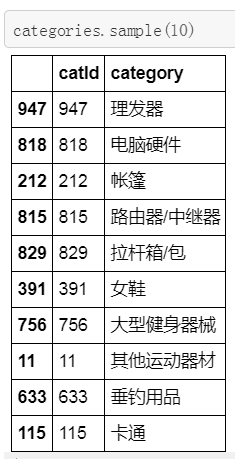
我们发现在categories表中罗列了所有的catId,但是并没有区分一级、二级、三级类目的标志。因此我们要从products表中的解析catIds字段,将原来混合在一起的三类目拆分为三个独立的类目,这样才有助于我们从中过滤出服装类的数据。如何解析catIds字段就不在这里详细说明了(源码中有),在这里让大家看一下解析好的products表:

我们将catIds分解成三个独立的字段,cat1,cat2,cat3分布对应一级类目、二级类目、三级类目,并将原来的catId都替换成了categories表中的类目名称,这样我们就不再需要categories表了。下面我们简单看一下一级类目cat1的数据分布情况:
d = {'cat1':products['cat1'].value_counts().index, 'count': products['cat1'].value_counts()}
df_cat1 = pd.DataFrame(data=d).reset_index(drop=True)

df_cat1.plot(x='cat1', y='count', kind='bar', legend=False,  figsize=(8, 5))
plt.title("cat1 分布")
plt.ylabel('count', fontsize=18)
plt.xlabel('cat1', fontsize=18)
在一级类目cat1的数据中"图书音像" 数据最多,但是数据也比较杂乱,因此这次我们选择“服饰服装”类数据来进行推荐
books = products[products.cat1=='图书音像']
clothes = products[products.cat1=='服饰服装']
computers = products[products.cat1=='电脑/办公']
sports = products[products.cat1=='运动户外']
Shoes= products[products.cat1=='鞋类箱包']
homelife= products[products.cat1=='家居生活']
mobile= products[products.cat1=='手机/数码']

#我们需要的是服装类数据
clothes = clothes[['productId','name']]
clothes = clothes.reset_index(drop=True)
print(len(clothes))
clothes.head(10)
处理数据
如何拆分products表中的catIds字段,这里不再说明,请看源代码,下面我们要对clothes表的name字段进行清洗,我们要删除一些符号,并进行分词,最后我们生成两新的字段:clean_name和cut_name。
#定义删各种符号的函数
def remove_punctuation(line):
    line = str(line)
    if line.strip()=='':
        return ''
    r = '[’!"#$%&\'()*+,-./:;<=>?@[\\]^_`{|}~]+'
    line = re.sub(r, '', line)
    return line

#删除各种符号
clothes['clean_name'] = clothes['name'].apply(remove_punctuation)
#分词
clothes['cut_name'] = clothes['clean_name'].apply(lambda x: " ".join([w for w in list(jb.cut(x)) if w !=' ']))
clothes.head()
数据分析
首先我们查看name中最常用的20个词语
def get_top_n_words(corpus, n=None):
    vec = CountVectorizer().fit(corpus)
    bag_of_words = vec.transform(corpus)
    sum_words = bag_of_words.sum(axis=0)
    words_freq = [(word, sum_words[0, idx]) for word, idx in vec.vocabulary_.items()]
    words_freq =sorted(words_freq, key = lambda x: x[1], reverse=True)
    return words_freq[:n]

common_words = get_top_n_words(clothes['cut_name'], 20)
df1 = pd.DataFrame(common_words, columns = ['cut_name' , 'count'])
df1.groupby('cut_name').sum()['count'].sort_values().iplot(kind='barh', yTitle='Count', linecolor='black', title='name中最常用的20个词语 ') 
接下来我们查看最常用的20个Bigrams词语对:
def get_top_n_bigram(corpus, n=None):
    vec = CountVectorizer(ngram_range=(2, 2)).fit(corpus)
    bag_of_words = vec.transform(corpus)
    sum_words = bag_of_words.sum(axis=0)
    words_freq = [(word, sum_words[0, idx]) for word, idx in vec.vocabulary_.items()]
    words_freq =sorted(words_freq, key = lambda x: x[1], reverse=True)
    return words_freq[:n]
common_words = get_top_n_bigram(clothes['cut_name'], 20)
df2 = pd.DataFrame(common_words, columns = ['cut_name' , 'count'])
df2.groupby('cut_name').sum()['count'].sort_values(ascending=False).iplot(kind='bar', yTitle='Count', linecolor='black', title='最常用的20个Bigrams词语对')
最后我们查看一下最常用的20个Trigrams词语对
def get_top_n_trigram(corpus, n=None):
    vec = CountVectorizer(ngram_range=(3, 3)).fit(corpus)
    bag_of_words = vec.transform(corpus)
    sum_words = bag_of_words.sum(axis=0)
    words_freq = [(word, sum_words[0, idx]) for word, idx in vec.vocabulary_.items()]
    words_freq =sorted(words_freq, key = lambda x: x[1], reverse=True)
    return words_freq[:n]
common_words = get_top_n_trigram(clothes['cut_name'], 20)
df5 = pd.DataFrame(common_words, columns = ['cut_name' , 'count'])
df5.groupby('cut_name').sum()['count'].sort_values(ascending=False).iplot(kind='bar', yTitle='Count', linecolor='black', title='最常用的20个Trigrams词语对') 
接下来我们查看一下name中词语数量的分布:
clothes['word_count'] = clothes['cut_name'].apply(lambda x: len(str(x).split()))

name_lengths = list(clothes['word_count'])

print("name数量:",len(name_lengths),
      "\nname平均词语数", np.average(name_lengths),
      "\nname最少词语数", min(name_lengths),
      "\nname最多词语数", max(name_lengths))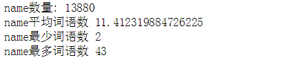
clothes['word_count'].iplot(
    kind='hist',
    bins = 50,
    linecolor='black',
    xTitle='word count',
    yTitle='count',
title='name的词语数量的分布') 
我们看到大部分name的所包含的词语数量在6至15个之间。
推荐模型
首先我们要对经过分词的cut_name字段进行向量化处理,在这里我们使用sklearn的TfidfVectorizer来对文本数据进行向量化处理。
tfidf  = TfidfVectorizer(analyzer='word', ngram_range=(1, 2), min_df=0).fit(clothes['cut_name'])
tfidf_vec = tfidf.transform(clothes['cut_name'])
然后我们定义一个处理文本的函数,该函数的功能是将特定name进行清洗和分词,以便系统根据特定name来推荐与其相似的其他的服装,同样也可以处理用户输入的自定义name.
def processText(text):
    text = str(text)
    if text.strip()=='':
        return ''
    r = '[’!"#$%&\'()*+,-./:;<=>?@[\\]^_`{|}~]+'
    text = re.sub(r, '', text)
    text = [",".join([w for w in list(jb.cut(text)) if w !=' '])]
    return text
接下来我们创建一个推荐函数,该函数通过余弦相似度来匹配与特定name相似的其他n个服装,并将推荐结果返回给用户:
def recommendations(text,num):
    ss = processText(text)
    ss_vec = tfidf.transform(ss)
    cos_sim = cosine_similarity(ss_vec, tfidf_vec)
    arr =cos_sim[0]
    idxs=list(np.argsort(-arr)[:num])
    for idx in idxs:
        row = clothes[clothes.index==idx]
        productId = row.productId.values[0]
        name = row.name.values[0]
        print("productId:",productId,",",name)
最后让我们来看一下基于内容的服装推荐的效果吧,我们从clothes表中随机选几个商品的name,然后让系统根据这些name来推荐10个与其相似的别的服装。

最后我们看一下自定义name的推荐效果:


总结
基于内容的推荐可以利用产品的元数据,如名称、规格或技术参数等进行推荐,而不依赖用户的行为数据如评分,点击记录等。这样可以有效的解决冷启动的问题。
可以点击这里查看代码中图表的交互效果
完整代码在这里下载