SAS GTL 散点图

libname a '.\data';

 

data scatter;

    set a.scatter;

run;

 

proc template;

    define statgraph scatter;

       dynamic ht wt;

       mvar study;

       begingraph /border=false designwidth=wt designheight=ht;

           layout overlay/cycleattrs=true xaxisopts=(label='Peak X' labelattrs=(size=9pt) type=log logopts=(minorticks=true minortickcount=1 viewmin=0.1 base=10 tickintervalstyle=logexpand ) tickvalueattrs=(size=9pt) )

                                     yaxisopts=(label='Peak Y' labelattrs=(size=9pt) type=log logopts=(minorticks=true minortickcount=8 viewmin=0.1 base=10 tickintervalstyle=logexpand) tickvalueattrs=(size=9pt))

 

;

               scatterplot x=alt1 y=bili1/name='legend1' datalabel=datalabel datalabelattrs=(size=6pt) markerattrs=(symbol=circle color=red);

               scatterplot x=alt2 y=bili2 /name='legend2' datalabel=datalabel datalabelattrs=(size=6pt) markerattrs=(symbol=triangle color=blue);

               referenceline y=2/lineattrs=(pattern=2) curvelabelattrs=(size=8pt) curvelabellocation=outside curvelabelposition=max curvelabel='2xULN';

               referenceline x=3/lineattrs=(pattern=2) curvelabelattrs=(size=8pt) curvelabellocation=outside curvelabelposition=max curvelabel='3xULN';

               discretelegend 'legend1' 'legend2' /border=false ;

           endlayout;

       endgraph;

    end;

run;

 

option orientation=landscape nodate nonumber nobyline;

ods _all_ close;

ods listing;

 

ods graphics on/reset=index;

 

title1 h=1 j=l 'Stydy' j=r 'Protocol';

title2 h=1 j=l "Study:102 Data Cutoff:&systime" j=r "Data Extract:&systime";

title3 j=c 'Figure 1 Tumor';

footnote1 j=l 'Valued for TLS';

footnote2 j=l "Source %sysfunc(TODAY(),DATE9.):&systime";

 

ods rtf file="scatter.rtf";

ods pdf file="scatter.pdf";

 

proc sgrender data=scatter template=scatter;

    dynamic ht='5.5in' wt='9in';

run;

 

ods pdf close;

ods rtf close;

ods graphics off;
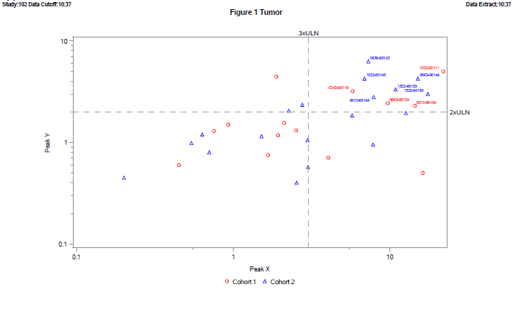
效果图
猜你喜欢
