机器学习技法 之 聚合模型（Aggregation Model）

聚合模型实际上就是将许多模型聚合在一起，从而使其分类性能更佳。

aggregation models: mix or combine hypotheses (for better performance)

下面举个例子：
你有 $T$ 朋友，他们对于股票涨停的预测表现为 $g_1,\cdots ,g_T$。 常见的聚合（aggregation）方法有：

1. select the most trust-worthy friend from their usual performance
   根据他们的平常表现，选出最值得信任的朋友
   $G(\mathbf{x})=g_{t_{*}}(\mathbf{x}) \text { with } t_{*}=\operatorname{argmin}_{t \in\{1,2, \ldots, T\}} E_{\text {val }}\left(g_{t}^{-}\right)$
2. mix the predictions from all your friends uniformly
   将所有朋友的预测取平均值
   $G(\mathbf{x})=\operatorname{sign}\left(\sum_{t=1}^{T} 1 \cdot g_{t}(\mathbf{x})\right)$
3. mix the predictions from all your friends non-uniformly
   将所有朋友的预测值取加权平均值
   $G(\mathbf{x})=\operatorname{sign}\left(\sum_{t=1}^{T} \alpha_{t} \cdot g_{t}(\mathbf{x})\right) \text { with } \alpha_{t} \geq 0$
4. combine the predictions conditionally
   根据当前状态 $\mathbf{x}$ 确定权重后结合。
   $G(\mathbf{x})=\operatorname{sign}\left(\sum_{t=1}^{T} q_{t}(\mathbf{x}) \cdot g_{t}(\mathbf{x})\right) \text { with } q_{t}(\mathbf{x}) \geq 0$

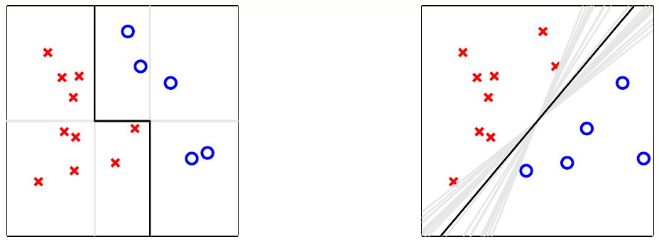
学到这里，可能有一种感觉，与模型选择比较相近，并根据直观印象，取平均获得是分类器一定比最好的差，比最差的好。所以会感觉 aggregation 用处不大，那现在看一下， aggregation 的真正的用处是什么？

以下图为例：

左侧第一个图中，实际上是使用三条竖线或横线实现了二分类，虽然竖线或横线是很弱的一种分类器，但是如此结合便获得了一个较强的分类器，其分类效果好于任何一个分类器独自分类的结果。

右侧第一个图中，是许多直线的取平均值获得的，这种状态存在于数据样本较少时，可以获取一种与SVM类似的效果，虽然这么多直线对于训练样本（采样数据）的分类效果一样，但是对于测试样本（全局数据）可能有更好的分类效果。

所以说真正的 aggregation 并不只是单纯的取平均而已，其可能是为了弥补当前分类器的不足（分类器分类性能较弱，分类器的泛化能力较弱）。即合理的聚合（aggregation）代表了更好的性能（performance）。

Blending

均值融合（uniform blending）

用于分类：

数学表达如下：

$G(\mathbf{x})=\operatorname{sign} \left( \sum_{t=1}^{T} g_{t}(\mathbf{x}) \right)$

有 $T$ 个人，每人一票。当 $g_{t}$ 预测值相近，那么性能不变。当 $g_{t}$ 多样民主时，少数服从多数（majority can correct minority）

在多分类中的数学表达为：

$G(\mathbf{x})=\underset{1 \leq k \leq K}{\operatorname{argmax}} \sum_{t=1}^{T}\left[\kern-0.15em\left[g_{t}(\mathbf{x})=k\right]\kern-0.15em\right]$

用于回归：

$G(\mathbf{x})=\frac{1}{T} \sum_{t=1}^{T} g_{t}(\mathbf{x})$

当 $g_{t}$ 预测值相近，那么性能不变。当 $g_{t}$ 多样民主时，一些分类结果 $g_{t}(\mathbf{x})>f(\mathbf{x})$ ，另一些分类结果 $g_{t}(\mathbf{x})<f(\mathbf{x})$，那么理想状态取平均可以获得最佳解。

综合上述两种需求，多样性的 hypotheses 更容易使得融合模型性能更佳。

现在进行理论分析，其性能是否改善，这里以回归模型为例：
这里的取平均是针对全部的 hypothesis 或者说 $T$ 个 $g_t$ 进行的，并针对的是随机的单个样本。
$\begin{aligned} \operatorname{avg}\left(\left(g_{t}(\mathrm{x})-f(\mathrm{x})\right)^{2}\right) &=\operatorname{avg}\left(g_{t}^{2}-2 g_{t} f+f^{2}\right) \\ &=\operatorname{avg}\left(g_{t}^{2}\right)-2 G f+f^{2} \\ &=\operatorname{avg}\left(g_{t}^{2}\right)-G^{2}+(G-f)^{2} \\ &=\operatorname{avg}\left(g_{t}^{2}\right)-2 G^{2}+G^{2}+(G-f)^{2} \\ &=\operatorname{avg}\left(g_{t}^{2}\right)-2\operatorname{avg}\left(g_{t}\right)G+G^{2}+(G-f)^{2} \\ &=\operatorname{avg}\left(g_{t}^{2}-2 g_{t} G+G^{2}\right)+(G-f)^{2} \\ &=\operatorname{avg}\left(\left(g_{t}-G\right)^{2}\right)+(G-f)^{2} \end{aligned}$

也就是说，在对全部训练样本 $\mathbf{x}_n$ 进行分析取全部误差的平均值。这里 用 $\mathcal{E}$ 表示平均值。举个例子： $\frac{1}{N}\sum_{n = 1}^{N}\left(g_{t}(\mathrm{x}_n)-f(\mathrm{x}_n)\right)^{2} = \mathcal{E}\left(g_{t}-f\right)^{2}$。

$\begin{aligned} \operatorname{avg}\left(\mathcal{E}\left(g_{t}-f\right)^{2}\right) &=\operatorname{avg}\left(\mathcal{E}\left(g_{t}-G\right)^{2}\right) & +\mathcal{E}(G-f)^{2}\\ \operatorname{avg}\left(E_{\text {out }}\left(g_{t}\right)\right) &=\operatorname{avg}\left(\mathcal{E}\left(g_{t}-G\right)^{2}\right) &+E_{\text {out }}(G) \\ & \geq & +E_{\text {out }}(G) \end{aligned}$

即 $G$ 优于 $g_t$ 的平均值。

现在假设在分布为 $P^{N}$ (i.i.d.) 的数据上选取大小为 $N$ 的数据集 $\mathcal{D}_{t}$，并通过 $\mathcal{A}\left(\mathcal{D}_{t}\right)$ 获取 $g_{t}$。那么执行无数次可以获取到 $\bar g$，表达式如下：

$\bar{g}=\lim _{T \rightarrow \infty} G=\lim _{T \rightarrow \infty} \frac{1}{T} \sum_{t=1}^{T} g_{t}=\underset{\mathcal{D}}{\mathcal{E}} \mathcal{A}(\mathcal{D})$

那么现在用 $\bar{g}$ 代替 $G$，之前所求仍然成立，即：

$\begin{aligned} \operatorname{avg}\left(E_{\text {out }}\left(g_{t}\right)\right) &=\operatorname{avg}\left(\mathcal{E}\left(g_{t}-\bar{g}\right)^{2}\right) &+E_{\text {out }}(\bar{g}) \\ \end{aligned}$

其中

• $\operatorname{avg}\left(E_{\text {out }}\left(g_{t}\right)\right)$ 代表了算法的期望性能（expected performance of A）。
• $E_{\text {out }}(\bar{g})$ 代表了共识性能（performance of consensus），又叫偏差（bias）
• $\operatorname{avg}\left(\mathcal{E}\left(g_{t}-\bar{g}\right)^{2}\right)$ 代表了共识的期望偏差（expected deviation to consensus），又叫方差（variance）

线性融合（Linear Blending）

用于分类：

数学表达如下：

$G(\mathbf{x})=\operatorname{sign}\left(\sum_{t=1}^{T} \alpha_{t} \cdot g_{t}(\mathbf{x})\right) \text { with } \alpha_{t} \geq 0$

与均值融合相似，有 $T$ 个人，但是每人 $\alpha_t$ 票，而不是都只有一票。

用于回归：
$\min _{\alpha_{t} \geq 0} \frac{1}{N} \sum_{n=1}^{N}\left(y_{n}-\sum_{t=1}^{T} \alpha_{t} g_{t}\left(\mathbf{x}_{n}\right)\right)^{2}$

这里重温一下线性回归加非线性转换的结合模型，其数学表达如下：

$\min _{w_{i}} \frac{1}{N} \sum_{n=1}^{N}\left(y_{n}-\sum_{i=1}^{\tilde{d}} w_{i} \phi_{i}\left(\mathbf{x}_{n}\right)\right)^{2}$

可以看出两种非常相似。

所以说线性融合就是线性回归使用假设函数作为非线性转换工具，并且有约束条件。

那么该最优化问题可以写为：
$\min _{\alpha_{t} \geq 0} \frac{1}{N} \sum_{n=1}^{N} \operatorname{err}\left(y_{n}, \sum_{t=1}^{T} \alpha_{t} g_{t}\left(\mathbf{x}_{n}\right)\right)$

在实际运用中，常常不用约束条件 $\alpha_t > 0$，因为：
$\text { if } \alpha_{t}<0 \Rightarrow \alpha_{t} g_{t}(\mathbf{x})=\left|\alpha_{t}\right|\left(-g_{t}(\mathbf{x})\right)$
也就是说认为 $g_t$ 的分类错误很高，与预测值常常相反。那么取反便会得到较好性能的分类器。

与模型选择一样，虽然使用训练集获取 $g_t$，但是最好使用验证集获取 $\alpha_t$。

堆叠融合（Stacking or Any Blending）

前面提到的均值融合和线性融合实际上类似于滤波，将预测值乘以一个系数后输出，若将其视为一个模型，那么该模型表达式为 $\tilde g(g_1,g_2,\cdots,g_T) = \alpha_1 g_1 + \alpha_2 g_2 + \cdots + \alpha_T g_T$。那么 blending 的一般形式便不局限于输入参数的线性组合，可能 $\tilde g$ 是也是一个 hypothesis。

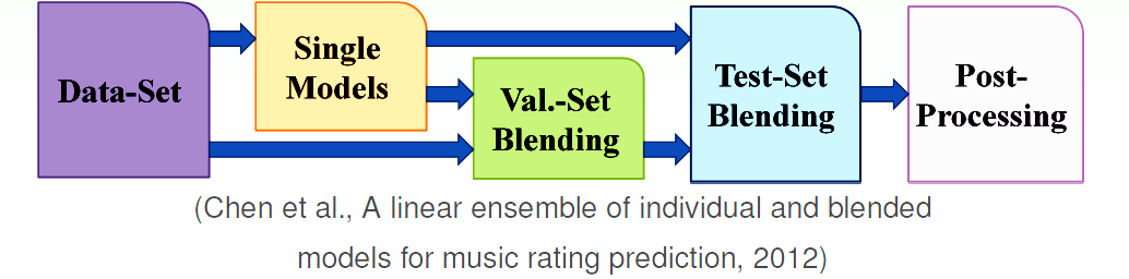
Given $g_{1}^{-}, g_{2}^{-}, \ldots, g_{T}^{-}$ from $\mathcal{D}_{\text {train }},$ transform $\left(\mathbf{x}_{n}, y_{n}\right)$ in $\mathcal{D}_{\text {val }}$ to $\left(\mathbf{z}_{n}=\Phi^{-}\left(\mathbf{x}_{n}\right), y_{n}\right),$ where

学习步骤如下：

1. 从训练集 $\mathcal{D}_{\text {train}}$ 中获取 $g_{1}^{-}, g_{2}^{-}, \ldots, g_{T}^{-}$，将验证集数据映射到 $\mathcal Z$ 空间，即 $\mathbf{z}_{n}=\left(\Phi^{-}\left(\mathbf{x}_{n}\right), y_{n}\right)$ ，其中映射函数为： $\Phi^{-}(\mathbf{x})=\left(g_{1}^{-}(\mathbf{x}), \ldots, g_{T}^{-}(\mathbf{x})\right)$
2. 在 $\mathcal{Z}$ 空间训练出融合各种模型的模型（函数） $\tilde{g}$ $=$ AnyModel $\left(\left\{\left(\mathbf{z}_{n}, y_{n}\right)\right\}\right)$
3. 最终的堆叠融合模型 $G_{\mathrm{ANYB}}(\mathbf{x})=\tilde{g}(\Phi(\mathbf{x}))$。

优缺点：

• 很强大（powerful），可以完成有条件的融合（conditional blending）
• 很容易过拟合（模型复杂度过高）

应用（Blending in Practice）

在 any blending 的基础上，将原来的 $g_t$ 和 $G$ 结合在一起再做一次融合。

Bagging

blending : 在获取 $g_t$ 之后，进行聚合;
learning : 在聚合（学习）过程中获取 $g_t$。

获得多样 $g_t$ 的方法有：

• diversity by different models
• diversity by different parameters: 例如优化方法GD的步长变化多样
• diversity by algorithmic randomness
• diversity by data randomness

下面便从数据出发，来满足假设函数的多样性。

那应该怎么做呢，在前面提到有共识便是一个模型的期望表现：

$\text { consensus } \bar { g } = \text { expected } g _ { t } \text { from } \mathcal { D } _ { t } \sim P ^ { N }$

其优于单个的 $g_t$。

其由两个部分组成，一个是无穷多个 $g_t$，另一个则是丰富的样本数据。对于第一个问题这里提供有限个但相当多个 $g_t$，第二个问题只能从手中的数据入手，来创造多样的样本数据集 $\mathcal{D}_t$。

拔靴法（Bootstrap Aggregation）

Bagging 实际上就是指 Bootstrap Aggregation，拔靴法实际上是从手中的数据重采样来获得仿真的 $\mathcal{D}_t$。其实现方法是：

1. 在原有的大小为 $N$ 的数据集 $\mathcal{D}$ 上，有放回的采样 $N^\prime$ 次获得仿真数据集 $\tilde \mathcal{D} _ t \rightarrow$ 这一步便是 Bootstrap 操作。
2. 通过 $\mathcal A (\tilde \mathcal{D} _ t)$ 获取 $g_t$，再使用均值融合获得： $G = \operatorname {Uniform}(\{g_t\})$。

拔靴法（bootstrap aggregation）是一种简单的基于基算法（base algorithm $\mathcal A$）的融合算法（meta algorithm）。方法合理前提是：数据集的多样性和基算法 $\mathcal A$ 对于随机数据敏感。

Adaptive Boosting

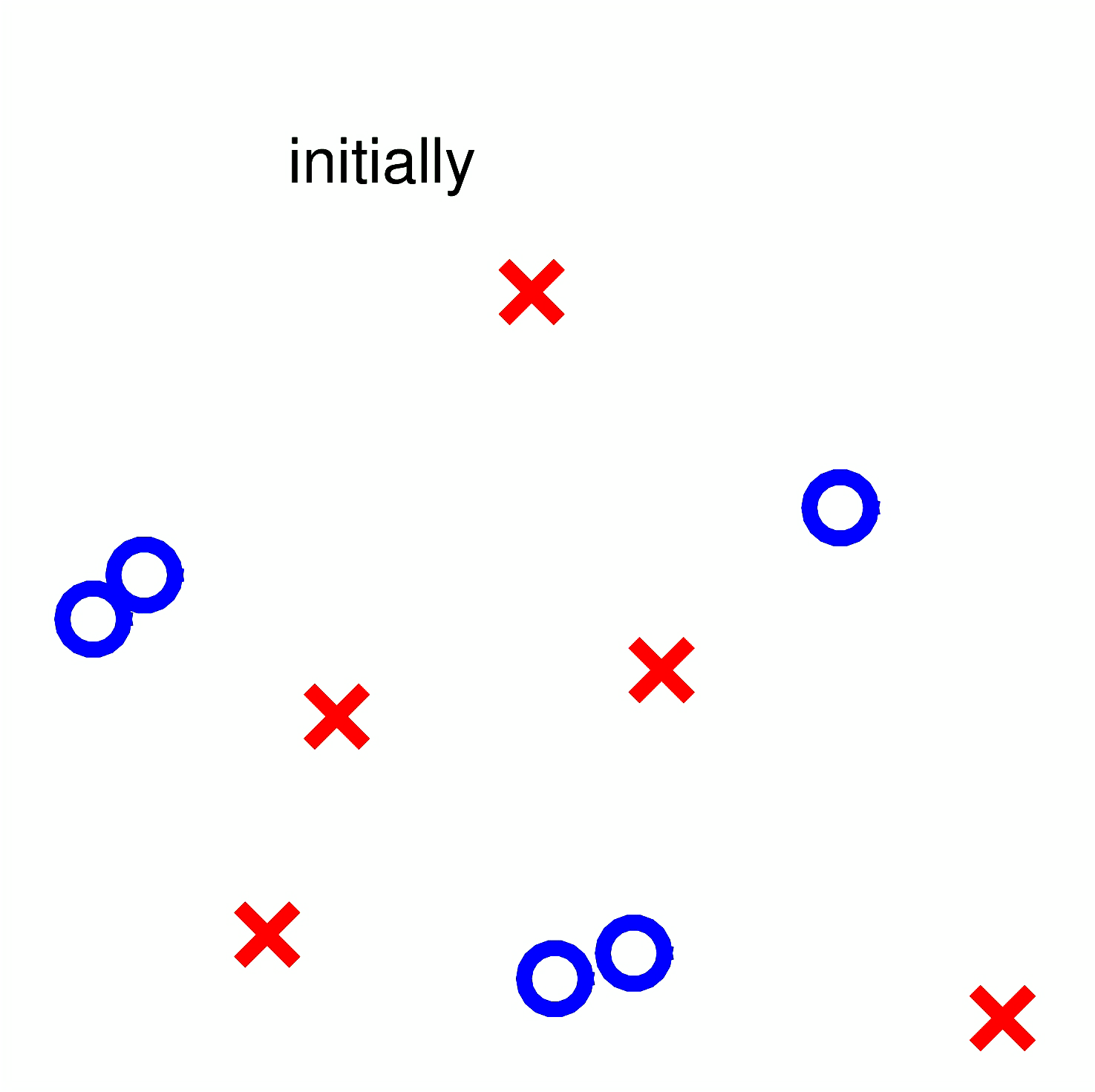
Adaptive Boosting （AdaBoost ）实际上是从 Bagging 的核心 bootstrap 出发实现的一种融合算法。具体实现如下：

加权基算法（Weighted Base Algorithm）

数据集的构造相当于对于不同样本的权重不同，也就是说重采样（Re-sample）过程相当于重赋予权重（Re-weighting）过程：

假设重采样如下：

$\begin{aligned} \mathcal { D } = \left\{ \left( \mathbf { x } _ { 1 } , y _ { 1 } \right) , \left( \mathbf { x } _ { 2 } , y _ { 2 } \right) , \left( \mathbf { x } _ { 3 } , y _ { 3 } \right) , \left( \mathbf { x } _ { 4 } , y _ { 4 } \right) \right\} \\ \stackrel { \text { bootstrap } } { \Longrightarrow } \tilde { \mathcal { D } } _ { t } = \left\{ \left( \mathbf { x } _ { 1 } , y _ { 1 } \right) , \left( \mathbf { x } _ { 1 } , y _ { 1 } \right) , \left( \mathbf { x } _ { 2 } , y _ { 2 } \right) , \left( \mathbf { x } _ { 4 } , y _ { 4 } \right) \right\} \end{aligned}$

原来的误差计算如下：
$E _ { \mathrm { in } } ^ { 0 / 1 } ( h ) = \frac { 1 } { 4 } \sum _ { ( \mathbf { x } , y ) \in \tilde { D } _ { t } } \left[\kern-0.15em\left[ y \neq h ( \mathbf { x } ) \right]\kern-0.15em\right]$

现在则是：

$E _ { \mathrm { in } } ^ { \mathrm { u }^{(t)} } ( h ) = \frac { 1 } { 4 } \sum _ { n = 1 } ^ { 4 } u _ { n } ^ { ( t ) } \cdot \left[\kern-0.15em\left[ y _ { n } \neq h \left( \mathbf { x } _ { n } \right) \right]\kern-0.15em\right]$

其中 $u_1 = 2,u_2 = 1,u_3 = 0,u_4 = 1$。

那么袋中的每一个 $g_t$ 都是通过最小化加权误差（bootstrap-weighted error）获得的。

所以加权基算法（Weighted Base Algorithm）的数学表达为：

$E _ { \mathrm { in } } ^ { \mathrm { u } } ( h ) = \frac { 1 } { N } \sum _ { n = 1 } ^ { N } u _ { n } \cdot \operatorname { err } \left( y _ { n } , h \left( \mathbf { x } _ { n } \right) \right)$

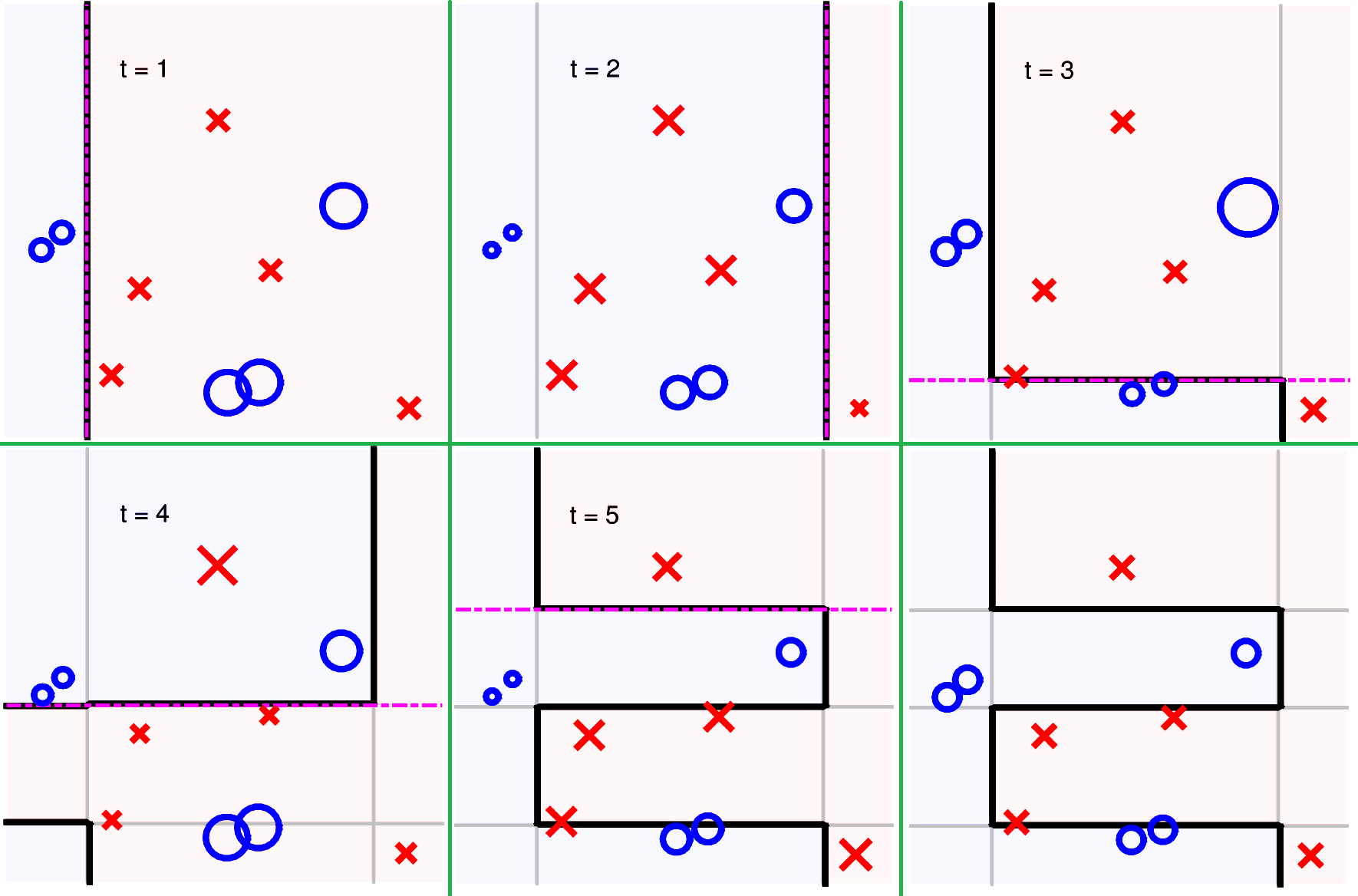
那么通过重新赋值获取多样的 $g_t$ 是另一种可行的方法：

假如两个 $g_t$ 的获取方法如下：
$\begin{aligned} g _ { t } & \leftarrow \underset { h \in \mathcal { H } } { \operatorname { argmin } } \left( \sum _ { n = 1 } ^ { N } u _ { n } ^ { ( t ) } \left[ \kern-0.15em \left[ y _ { n } \neq h \left( \mathbf { x } _ { n } \right) \right]\kern-0.15em\right] \right) \\ g _ { t + 1 } & \leftarrow \underset { h \in \mathcal { H } } { \operatorname { argmin } } \left( \sum _ { n = 1 } ^ { N } u _ { n } ^ { ( t + 1 ) } \left[ \kern-0.15em \left[ y _ { n } \neq h \left( \mathbf { x } _ { n } \right) \right]\kern-0.15em\right] \right) \end{aligned}$

什么时候两个人分类器会很不一样呢？就是当 $g_t$ 对于权重 $u _ { n } ^ { ( t ) }$ 的性能很好，但是 $g_t$ 对于权重 $u _ { n } ^ { ( t + 1) }$ 的性能很差，最差的 $g$ 则是随机值也就是说有 50% 的概率会预测准确。即：

$\frac {\sum _ { n = 1 } ^ { N } u _ { n } ^ { ( t + 1 ) } \left[ \kern-0.15em \left[y _ { n } \neq g _ { t } \left( \mathbf { x } _ { n } \right) \right] \kern-0.15em \right] } { \sum _ { n = 1 } ^ { N } u _ { n } ^ { ( t + 1 ) } } = \frac { 1 } { 2 }$

所以现在希望的效果是：

$\frac {\sum _ { n = 1 } ^ { N } u _ { n } ^ { ( t + 1 ) } \left[ \kern-0.15em \left[y _ { n } \neq g _ { t } \left( \mathbf { x } _ { n } \right) \right] \kern-0.15em \right] } { \sum _ { n = 1 } ^ { N } u _ { n } ^ { ( t + 1 ) } } = \frac { \square_ { t + 1 } } { \square_ { t + 1 } + \bigcirc_{ t + 1 } } = \frac { 1 } { 2 } , \text { where } \\ \square_ { t + 1 } = \sum _ { n = 1 } ^ { N } u _ { n } ^ { ( t + 1 ) } \left[ \kern-0.15em \left[y _ { n } \neq g _ { t } \left( \mathbf { x } _ { n } \right) \right] \kern-0.15em \right]\\ \bigcirc_{ t + 1 } = \sum _ { n = 1 } ^ { N } u _ { n } ^ { ( t + 1 ) } \left[ \kern-0.15em \left[y _ { n } = g _ { t } \left( \mathbf { x } _ { n } \right) \right] \kern-0.15em \right]$

那么通过重新放缩权重（re-scaling (multiplying) weights）便可以实现，即：

对于 $g_t$ 分类错误的样本：

$u _ { n } ^ { ( t + 1 ) } = \bigcirc_{ t } \cdot u _ { n } ^ { ( t ) }$

对于 $g_t$ 分类正确的样本：

$u _ { n } ^ { ( t + 1 ) } = \square_{ t } \cdot u _ { n } ^ { ( t ) }$

那么在实际中如何实现呢？这里提出放缩系数。

放缩系数（Scaling Factor）

错误率 $\epsilon _ { t }$ 定义如下：
$\epsilon _ { t } = \frac {\sum _ { n = 1 } ^ { N } u _ { n } ^ { ( t ) } \left[ \kern-0.15em \left[y _ { n } \neq g _ { t } \left( \mathbf { x } _ { n } \right) \right] \kern-0.15em \right] } { \sum _ { n = 1 } ^ { N } u _ { n } ^ { ( t) } }$

放缩系数的定义如下：
$\mathbf { \star } _ { t } = \sqrt { \frac { 1 - \epsilon _ { t } } { \epsilon _ { t } } }$

那么：

$\begin{aligned} \left[ \kern-0.15em \left[y _ { n } \neq g _ { t } \left( \mathbf { x } _ { n } \right) \right] \kern-0.15em \right] \quad u ^ { ( t + 1 ) } _ n &\leftarrow u ^ { ( t ) } _ n \cdot \mathbf { \star } _ { t } \\ \left[ \kern-0.15em \left[y _ { n } = g _ { t } \left( \mathbf { x } _ { n } \right) \right] \kern-0.15em \right] \quad u ^ { ( t + 1 ) } _ n &\leftarrow u ^ { ( t ) } _n / \mathbf { \star } _ { t } \end{aligned}$

Linear Aggregation on the Fly

有了上述的前提，便可以设计一个由数据多样化创造的融合算法，而AdaBoost 除了上述一些前提外，还有一步，那就是 Linear Aggregation on the Fly，在学习中获得线性融合的参数 $\alpha_t$，即：

$\alpha_t = \ln(\mathbf { \star } _ { t })$

1. 当 $\epsilon _ { t } \rightarrow 0$ 时， $\mathbf { \star } _ { t } \rightarrow \inf, \ln(\mathbf { \star } _ { t }) \rightarrow \inf$，也就是说当无错误时，给予无穷权重，即当前 $g_t$ 完全可以完成任务。
2. 当 $\epsilon _ { t } = \frac{1}{2}$ 时， $\mathbf { \star } _ { t } = 1, \ln(\mathbf { \star } _ { t }) = 0$也就是说当错误率为1/2时，不给予权重，即 $g_t$ 与随机数的性能一样无用。
3. 当 $\epsilon _ { t } \rightarrow 1$ 时， $\mathbf { \star } _ { t } = 0, \ln(\mathbf { \star } _ { t }) \rightarrow -\inf$ 也就是说当全错误时，给予负无穷权重，即只需要将分类结果取反便可以获得非常高准确率的 $g_t$。

AdaBoost 实现步骤

$u^{(1)} = \left[\frac{1}{N},\cdots,\frac{1}{N}\right]$
for $t = 1,\cdots,T$

1. 由 $\mathcal { A } \left( \mathcal { D } , \mathbf { u } ^ { ( t ) } \right)$ 获取 $g _ { t }$ ， 其中 $\mathcal { A }$ 用于优化权重为 $\mathbf { u } ^ { ( t ) }$ 的加权误差。

2. 由 $\mathbf { u } ^ { ( t ) }$ 更新 $\mathbf { u } ^ { ( t+1 ) }$
   $\begin{aligned} \left[ \kern-0.15em \left[y _ { n } \neq g _ { t } \left( \mathbf { x } _ { n } \right) \right] \kern-0.15em \right] \quad u ^ { ( t + 1 ) } _ n &\leftarrow u ^ { ( t ) } _ n \cdot \mathbf { \star } _ { t } \\ \left[ \kern-0.15em \left[y _ { n } = g _ { t } \left( \mathbf { x } _ { n } \right) \right] \kern-0.15em \right] \quad u ^ { ( t + 1 ) } _ n &\leftarrow u ^ { ( t ) } _n / \mathbf { \star } _ { t } \end{aligned}$

   其中: $\epsilon _ { t } = \frac {\sum _ { n = 1 } ^ { N } u _ { n } ^ { ( t + 1 ) } \left[ \kern-0.15em \left[y _ { n } \neq g _ { t } \left( \mathbf { x } _ { n } \right) \right] \kern-0.15em \right] } { \sum _ { n = 1 } ^ { N } u _ { n } ^ { ( t + 1 ) } }$， $\mathbf { \star } _ { t } = \sqrt { \frac { 1 - \epsilon _ { t } } { \epsilon _ { t } } }$

3. 计算线性融合系数 $\alpha_t = \ln(\mathbf { \star } _ { t })$

4. 获得最终hypothesis： $G ( \mathbf { x } ) = \operatorname { sign } \left( \sum _ { t = 1 } ^ { T } \alpha _ { t } g _ { t } ( \mathbf { x } ) \right)$

理论证明（Theoretical Guarantee）

AdaBoost 的 VC bound 如下：
$E _ { \mathrm { out } } ( G ) \leq E _ { \mathrm { in } } ( G ) + O ( \sqrt { \underbrace { O \left( d _ { \mathrm { vc } } ( \mathcal { H } ) \cdot T \log T \right) }_{d_{\mathbf{vc}} \text{ of all possible } G} \cdot \frac { \log N } { N } } )$

原作者有证明最多经过 $T= \log(N)$ 次迭代，便可以实现 $E_{\text{in}}(G) = 0$，只要基模型比随机数性能优越即可 $\epsilon _ { t } \leq \epsilon < \frac { 1 } { 2 }$。

也就是说，如果基模型 $g$ 很弱（weak），但是总比随机数优秀，那么由AdaBoost + $\mathcal A$ 获取的 $G$ 也会很强（strong）。

决策树桩（Decision Stump）

数学表达如下：
$h _ { s , i , \theta } ( \mathbf { x } ) = s \cdot \operatorname { sign } \left( x _ { i } - \theta \right)$

一共有三个参数 特征（feature） $i$，阈值（threshold） $\theta$ ，方向（direction） $s$。其实现的功能便是一个分界点，特征（feature） $i$ 表达的是在第 $i$ 维的分解点，阈值（threshold） $\theta$ 代表在本维度的分界点位于 $\theta$，方向（direction） $s$ 代表了分界点两边的样本类型。

这是一个弱模型，但是将其作为 AdaBoost 的基模型便可以实现高精度预测了，并且效率很高，时间复杂度为： $O(d \cdot N \log N)$

若使用 Decision Stump 作为 AdaBoost 的基模型，假设一个简单的数据集如下分布：

那么其学习过程的一种状态可能如下表达：