机器学习实战：小麦种子（封装函数进行调参、标准化、绘图查看数据分布）

声明：内容非原创，代码来自葁sir

import numpy as np
import pandas as pd
import matplotlib.pyplot as plt
%matplotlib inline

# 导入数据集
seeds = pd.read_csv('data/seeds.csv',sep = '\t',header = None)
seeds.head()

	0	1	2	3	4	5	6	7
0	15.26	14.84	0.8710	5.763	3.312	2.221	5.220	Kama
1	14.88	14.57	0.8811	5.554	3.333	1.018	4.956	Kama
2	14.29	14.09	0.9050	5.291	3.337	2.699	4.825	Kama
3	13.84	13.94	0.8955	5.324	3.379	2.259	4.805	Kama
4	16.14	14.99	0.9034	5.658	3.562	1.355	5.175	Kama

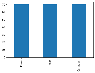
# 观察小麦有多少类
seeds[7].value_counts()

Kama        70
Rosa        70
Canadian    70
Name: 7, dtype: int64

seeds[7].value_counts().plot(kind = 'bar')

<AxesSubplot:>

# 或者用seaborn 
import seaborn as sns
sns.set()

# seaborn 常用图像
# barplot()
# scatterplot()
# swanrmplot()
# boxplot()
# violinplot()
# countplot()
# pairplot()
# heatmap()

from sklearn.model_selection import train_test_split
from sklearn.linear_model import Lasso,RidgeClassifier
from sklearn.neighbors import KNeighborsClassifier
from sklearn.tree import DecisionTreeClassifier
from sklearn.preprocessing import MinMaxScaler,StandardScaler

X = seeds.iloc[:,:7].copy()
# X = seeds.values[:,:7].copy() # 但是这样复制 numpy.ndarray
X.shape

(210, 7)

X

	0	1	2	3	4	5	6
0	15.26	14.84	0.8710	5.763	3.312	2.221	5.220
1	14.88	14.57	0.8811	5.554	3.333	1.018	4.956
2	14.29	14.09	0.9050	5.291	3.337	2.699	4.825
3	13.84	13.94	0.8955	5.324	3.379	2.259	4.805
4	16.14	14.99	0.9034	5.658	3.562	1.355	5.175
...	...	...	...	...	...	...	...
205	12.19	13.20	0.8783	5.137	2.981	3.631	4.870
206	11.23	12.88	0.8511	5.140	2.795	4.325	5.003
207	13.20	13.66	0.8883	5.236	3.232	8.315	5.056
208	11.84	13.21	0.8521	5.175	2.836	3.598	5.044
209	12.30	13.34	0.8684	5.243	2.974	5.637	5.063

210 rows × 7 columns

y =  seeds.iloc[:,-1].copy()
# y = seeds.values[:,-1].copy()
y.shape

(210,)

X_train,X_test,y_train,y_test = train_test_split(X,y,test_size=0.2,random_state=1)

# 封装函数来进行knn试探性运算
def knn_score(k,X,y):
    # 构造算法对象
    knn = KNeighborsClassifier(n_neighbors = k)
    scores = []
    train_scores = []
    for i in range(100):
        # 拆分
        X_train,X_test,y_train,y_test = train_test_split(X,y,test_size=0.2,random_state=1)
        # 训练
        knn.fit(X_train,y_train)
        # 评价模型
        scores.append(knn.score(X_test,y_test))
        # 经验评分
        train_scores.append(knn.score(X_train,y_train))
        
    return np.array(scores).mean(),np.array(train_scores).mean()

# 调参
result_dict = {
    
    }
k_list = [1,3,5,7,9,11]
for k in k_list:
    score,train_score = knn_score(k,X,y)
    result_dict[k] = [score,train_score]
    

result_dict

{1: [0.9047619047619047, 1.0],
 3: [0.9047619047619047, 0.9642857142857139],
 5: [0.8571428571428572, 0.9285714285714287],
 7: [0.8571428571428572, 0.9345238095238096],
 9: [0.8809523809523812, 0.9226190476190478],
 11: [0.8809523809523812, 0.9226190476190478]}

pd.DataFrame(result_dict).T

	0	1
1	0.904762	1.000000
3	0.904762	0.964286
5	0.857143	0.928571
7	0.857143	0.934524
9	0.880952	0.922619
11	0.880952	0.922619

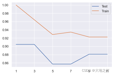
result = pd.DataFrame(result_dict).T.copy()

result.columns = ['Test','Train']

result

	Test	Train
1	0.904762	1.000000
3	0.904762	0.964286
5	0.857143	0.928571
7	0.857143	0.934524
9	0.880952	0.922619
11	0.880952	0.922619

result.plot()
plt.xticks(k_list)
plt.show()

进阶版

# z-score (x-x.mean)/ x.std  N(0,1)
# MinMaxScaller (x-x.min)/(x.max-x.min)  0-1

# 异常值 空值 数据分布查看

X.shape

(210, 7)

# 查看统计学指标
X.describe().T

	count	mean	std	min	25%	50%	75%	max
0	210.0	14.847524	2.909699	10.5900	12.27000	14.35500	17.305000	21.1800
1	210.0	14.559286	1.305959	12.4100	13.45000	14.32000	15.715000	17.2500
2	210.0	0.870999	0.023629	0.8081	0.85690	0.87345	0.887775	0.9183
3	210.0	5.628533	0.443063	4.8990	5.26225	5.52350	5.979750	6.6750
4	210.0	3.258605	0.377714	2.6300	2.94400	3.23700	3.561750	4.0330
5	210.0	3.700201	1.503557	0.7651	2.56150	3.59900	4.768750	8.4560
6	210.0	5.408071	0.491480	4.5190	5.04500	5.22300	5.877000	6.5500

def standard_X(X):
    X_copy = X.copy() # 拿数据
    for col_name in X_copy.columns: # 取列名
        col_data = X_copy[[col_name]] # 根据列名拿列数据，两个方括号是因为要二维数组
        # fit_transform
        stand_data = StandardScaler().fit_transform(col_data.values) # 标准化
        X_copy[col_name] = stand_data # 将数据替换成标准化后的数据
    return X_copy

standard_X(X).describe([0.01,0.25,0.5,0.75,0.99]).T
# standard_X(X).describe([0.01,0.25,0.5,0.75,0.99]).T

	count	mean	std	min	1%	25%	50%	75%	99%	max
0	210.0	-5.392512e-17	1.002389	-1.466714	-1.397504	-0.887955	-0.169674	0.846599	2.072913	2.181534
1	210.0	9.146123e-17	1.002389	-1.649686	-1.474607	-0.851433	-0.183664	0.887069	2.023505	2.065260
2	210.0	1.322091e-15	1.002389	-2.668236	-2.588824	-0.598079	0.103993	0.711677	1.678118	2.006586
3	210.0	-2.182910e-15	1.002389	-1.650501	-1.464372	-0.828682	-0.237628	0.794595	2.154459	2.367533
4	210.0	-2.030122e-16	1.002389	-1.668209	-1.634930	-0.834907	-0.057335	0.804496	1.936725	2.055112
5	210.0	-3.679596e-16	1.002389	-1.956769	-1.857934	-0.759148	-0.067469	0.712379	2.519905	3.170590
6	210.0	-1.337554e-16	1.002389	-1.813288	-1.633810	-0.740495	-0.377459	0.956394	2.130797	2.328998

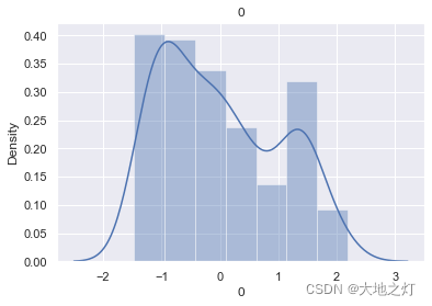
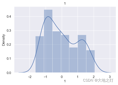
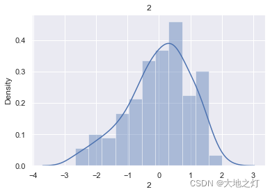
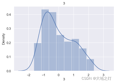
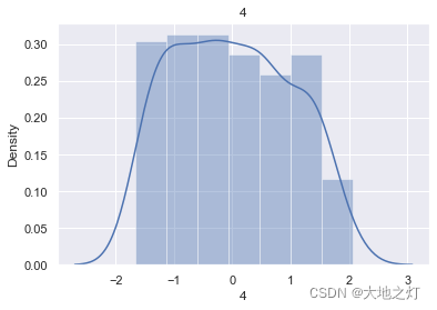
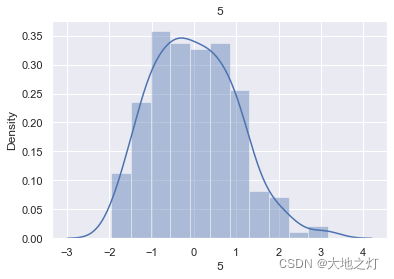
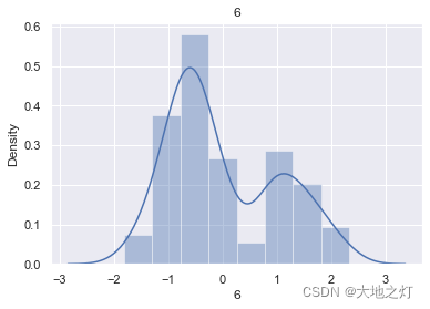
查看数据分布

经过对标准化数据describe查看99分位数 发现标签为2和5的两个列 有较大差距

stand_X = standard_X(X)

for col_name in stand_X.columns:
    sns.distplot(stand_X[col_name])
    plt.title(col_name)
    plt.show()

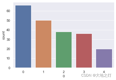
分箱操作

10 3000 5000 10000000

以5000为分割点 分割出高收入 低收入 进行映射 （减少数据之间的差异）

# 0 0 1 1 

X[0] = pd.cut(X[0],bins = 5,labels = [0,1,2,3,4])
# 将数据进行切割，防止过拟合

X[0]

0      2
1      2
2      1
3      1
4      2
      ..
205    0
206    0
207    1
208    0
209    0
Name: 0, Length: 210, dtype: category
Categories (5, int64): [0 < 1 < 2 < 3 < 4]

sns.countplot(X[0])

C:\Anaconda\lib\site-packages\seaborn\_decorators.py:36: FutureWarning: Pass the following variable as a keyword arg: x. From version 0.12, the only valid positional argument will be `data`, and passing other arguments without an explicit keyword will result in an error or misinterpretation.
  warnings.warn(





<AxesSubplot:xlabel='0', ylabel='count'>

# 拆所有数据
for col_name in X.columns:
    X[col_name] = pd.cut(X[col_name],bins = 5,labels = [0,1,2,3,4])

X

	0	1	2	3	4	5	6
0	2	2	2	2	2	0	1
1	2	2	3	1	2	0	1
2	1	1	4	1	2	1	0
3	1	1	3	1	2	0	0
4	2	2	4	2	3	0	1
...	...	...	...	...	...	...	...
205	0	0	3	0	1	1	0
206	0	0	1	0	0	2	1
207	1	1	3	0	2	4	1
208	0	0	1	0	0	1	1
209	0	0	2	0	1	3	1

210 rows × 7 columns

knn = KNeighborsClassifier()

X_train,X_test,y_train,y_test = train_test_split(X,y,test_size = 0.2,random_state = 1)

knn.fit(X_train,y_train)

KNeighborsClassifier()

knn.score(X_train,y_train)

0.9166666666666666

knn.score(X_test,y_test)

0.9523809523809523