机器学习应用之WebShell检测

本文主要参考自兜哥的《Web安全之机器学习入门》

前段时间在研究WebShell的检测查杀，然后看到兜哥的著作中提到的几个机器学习算法中也有实现WebShell检测的，主要有朴素贝叶斯分类、K邻近算法、图算法、循环神经网络算法等等，就一一试试看效果吧。

Python中的几个机器学习的库

1、numpy：

安装：pip install --user numpy

2、SciPy：

专为科学和工程设计的Python包，包括统计、优化、整合、线性代数模块、傅里叶变换、信号和图像处理、常微分方程求解器等。

安装：pip install --user numpy scipy matplotlib iPython jupyter pandas sympy nose

3、NLTK：

在NLP自然语言处理领域中最常用的一个Python库，包括图形演示和示例数据。

安装：pip install -U nltk

加载数据：

import nltk
nltk.download()

将提示要下载的包都下载安装完成即可。

用法示例：

分句：

import nltk
sent_tokenizer = nltk.data.load('tokenizers/punkt/english.pickle')
sentence = "This is the first sentence, and the second sentence is follow. This is the second sentence."
sentences = sent_tokenizer.tokenize(sentence)
print sentences

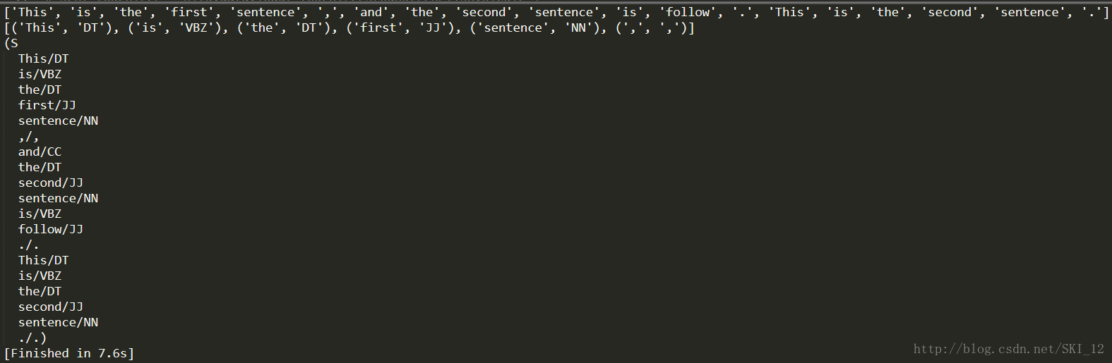
分词与标识、标识名词实体：

import nltk

sentence = "This is the first sentence, and the second sentence is follow. This is the second sentence."
tokens = nltk.word_tokenize(sentence)
print tokens

tagged = nltk.pos_tag(tokens)
print tagged[0:6]

entities = nltk.chunk.ne_chunk(tagged)
print entities

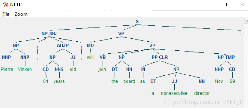
展现语法树：

from nltk.corpus import treebank
t = treebank.parsed_sents('wsj_0001.mrg')[0]
t.draw()

4、Scikit-Learn：

是基于Python的机器学习模块，基于BSD开源许可证，基本功能包括分类、回归、聚类、数据降维、模型选择、数据预处理等。

依赖的环境：

Python>=2.6 or >=3.3

NumPy>=1.6.1

SciPy>=0.9

安装：pip install -U scikit-learn

Scikit-Learn数据集：

最常见的是iris数据集，iris指鸢尾植物，其存储了其萼片和花瓣的长宽，共4个属性，且鸢尾植物又分为3类。iris里有两个属性：iris.data和iris.target。data里是一个矩阵，每一列代表了萼片或花瓣的长宽，共4列，一共采样150条记录；target是一个数组，存储了data中每条记录属于哪一类鸢尾植物，所以数组长度是150，不同的值只有3个。

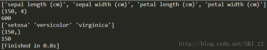
用法示例：

#coding=utf-8
from sklearn import datasets

iris = datasets.load_iris()

# iris.data共四列，一共采样150条记录；iris.target数组长度为150
print iris.feature_names # 显示特征名称
# print iris.data # 显示数据
print iris.data.shape
print iris.data.size # 显示数据的大小
# print iris.target
print iris.target_names # 显示分类名称
print iris.target.shape
print iris.target.size

特征提取：

1、数字型特征提取：

数字型特征是可以直接作为特征的，但可能存在少量的一些特征的取值范围较为异常，这时就需要进行预处理。常见的数字型特征预处理方法：

（1）标准化：

#coding=utf-8
from sklearn import preprocessing
import numpy as np

X = np.array([
	[1.,-1., 2.],
	[2., 0., 0.],
	[0., 1.,-1.]])

X_scaled = preprocessing.scale(X)
print X_scaled

（2）正则化：

#coding=utf-8
from sklearn import preprocessing

X = [[1.,-1., 2.],
	 [2., 0., 0.],
	 [0., 1.,-1.]]

X_normalized = preprocessing.normalize(X)
print X_normalized

（3）归一化：

#coding=utf-8
from sklearn import preprocessing
import numpy as np

X_train = np.array([
	[1.,-1., 2.],
	[2., 0., 0.],
	[0., 1.,-1.]])

min_max_scaler = preprocessing.MinMaxScaler()
X_train_minmax = min_max_scaler.fit_transform(X_train)
print X_train_minmax

2、文本性特征提取：

本质上是做单词切分，不同的单词当作一个新的特征。

#coding=utf-8
from sklearn.feature_extraction import DictVectorizer

measurements = [
	{'city': 'Dubai', 'temperature': 33.},
	{'city': 'London', 'temperature': 12.},
	{'city': 'San Fransisco', 'temperature': 18.},
]

vec = DictVectorizer()
array = vec.fit_transform(measurements).toarray()
feature_names = vec.get_feature_names()
print array
print feature_names

两个模型：词集模型和词袋模型。词集模型是单词构成的集合，集合中每个元素只有一个；词袋在词集的基础上增加了频率的维度，还记录了元素共有几个。

下一个示例是对一篇文章进行特征化，最常见的方式为词袋：

#coding=utf-8
from sklearn.feature_extraction.text import CountVectorizer

vectorizer = CountVectorizer(min_df=1)
print vectorizer

corpus = [
	'This is the first sentence.',
	'This is the second second sentence.',
	'And the third one.',
	'Is this the first sentence?'
]
X = vectorizer.fit_transform(corpus)
# 获取特征名称
print vectorizer.get_feature_names()
# 将现有的词袋特征进行向量化
print X.toarray()

# 针对其他文本进行词袋处理时，可以使用自定义的词袋的特征空间即词汇表
vocabulary = vectorizer.vocabulary_
new_vertorizer = CountVectorizer(min_df=1, vocabulary=vocabulary)
print new_vertorizer

3、数据读取：

#coding=utf-8
import tensorflow as tf
import numpy as np

# 从CSV文件中读取数据
training_set = tf.contrib.learn.datasets.base.load_csv_with_header(
	filename=" iris_training.csv",
	target_dtype=np.int,
	features_dtype=np.float32)
feature_columns = [tf.contrib.layers.real_valued_column("", dimension=4)]

# 访问数据集合的特征及标记
x = training_set.data
y = training_set.target

效果验证：

最常用的是交叉验证，这里以SVM为例：

#coding=utf-8
from sklearn.model_selection import train_test_split
from sklearn import datasets
from sklearn import svm

# 获取样本数据
iris = datasets.load_iris()
print iris.data.shape, iris.target.shape

# train_test_split()随机分割样本为训练样本和测试样本
X_train, X_test, y_train, y_test = train_test_split(iris.data, iris.target, test_size=0.4, random_state=0)
print "[*]The training sample:", X_train.shape, y_train.shape
print "[*]The test sample:", X_test.shape, y_test.shape

clf = svm.SVC(kernel='linear', C=1).fit(X_train, y_train)
print "[*]Accuracy rate:", clf.score(X_test, y_test)

这里使用train_test_split()函数随机分割样本为训练样本和测试样本，其中test_size参数指定测试样本在总样本所占的比例，random_state参数即指定随机状态。

为了提高验证的准确度，一般采用K折交叉验证。

K折交叉验证：初始采样分割成K个子样本，一个单独的子样本被保留作为验证模型的数据，其他K-1个样本用来训练。交叉验证重复K次，每个子样本验证一次，平均K次的结果或者使用其他结合方式，最终得到一个单一过程。

十折交叉验证示例：

#coding=utf-8
# 导入SVM库和datasets库
from sklearn import datasets
from sklearn import svm
# 导入K折交叉验证模块
from sklearn.model_selection import cross_val_score

# 获取样本数据
iris = datasets.load_iris()
print iris.data.shape, iris.target.shape
clf = svm.SVC(kernel='linear', C=1)
scores = cross_val_score(clf, iris.data, iris.target, cv=10)
print "[*]使用十折交叉验证："
print scores

将cross_val_score()函数中cv参数的值设置为3即为三折交叉验证：

朴素贝叶斯算法：

朴素贝叶斯（Naive Bayesian，NB），是贝叶斯分类算法的一种，是基于贝叶斯定理与特征条件独立假设的分类方法。

高斯朴素贝叶斯示例：

#coding=utf-8
from sklearn import datasets
iris = datasets.load_iris()
# 导入高斯朴素贝叶斯
from sklearn.naive_bayes import GaussianNB

# 训练数据集
gnb = GaussianNB()

# 验证结果
nb = gnb.fit(iris.data, iris.target) # 开始分类，对于量特别大的样本，可以使用函数partial_fit分类，避免一次加载过多数据到内存
y_pred = nb.predict(iris.data) # 参数为数组
# 比较y_pred数组和iris.target数组中不同元素的总个数
print "Number of mislabeled points out of a total %d points : %d" % (iris.data.shape[0], (iris.target != y_pred).sum())

1、检测WebShell（一）：

这里主要将遍历目录中所有的PHP文件，然后将每个PHP文件作为一个字符串进行处理，基于2-gram切割形成基于2-gram的词汇表。

至于书上本身的源代码在兜哥的Github上有，这里就不贴了，就附上该代码的运行结果，结果是使用三折交叉验证：

可以看到平均的准确率80%都不到，效果略差。

换为十折交叉验证试试看：

十折交叉验证的可信度更高，但明显看到效果更不好看，需要对匹配算法等进行改进才可以。

下面是个人修改过后的脚本，修改了黑样本库、换一个数量更多的PHP WebShell样本库，同时一下修改加载文件的方式：

#coding=utf-8
import os
from sklearn.feature_extraction.text import CountVectorizer
import sys
import numpy as np
from sklearn import cross_validation
from sklearn.naive_bayes import GaussianNB

def load_file(file_path):
	t = ""
	with open(file_path) as f:
		for line in f:
			line = line.strip('\n')
			t += line
	return t

def load_files(path):
	files_list = []
	for parent, dirs, files in os.walk(path):
		for file in files:
			if file.endswith('.php'):
				file_path = parent + '\\' + file
				print "[*]Loading: %s" % file_path
				t = load_file(file_path)
				files_list.append(t)
	return files_list

def main():
	# ngram_range设置为(2,2)表示以基于单词切割的2-gram算法生成词汇表因而token_pattern的正则为匹配单个单词，decode_error设置为忽略其他异常字符的影响，
	webshell_bigram_vectorizer = CountVectorizer(ngram_range=(2, 2), decode_error="ignore", token_pattern = r'\b\w+\b', min_df=1)
	# 加载WebShell黑样本
	webshell_files_list = load_files(u"E:\资料\Python\webshell-sample\webshell-master\webshell-master\php")
	# 将现有的词袋特征进行向量化
	x1 = webshell_bigram_vectorizer.fit_transform(webshell_files_list).toarray()
	y1 = [1] * len(x1)
	# 定义词汇表
	vocabulary = webshell_bigram_vectorizer.vocabulary_

	# vocabulary参数是使用黑样本生成的词汇表vocabulary将白样本特征化
	wp_bigram_vectorizer = CountVectorizer(ngram_range=(2, 2), decode_error="ignore", token_pattern = r'\b\w+\b', min_df=1, vocabulary=vocabulary)
	# 加载白样本
	wp_files_list = load_files(u"E:\资料\Python\\1book-master\data\wordpress")
	x2 = wp_bigram_vectorizer.fit_transform(wp_files_list).toarray()
	y2 = [0] * len(x2)

	# 拼接数组
	x = np.concatenate((x1, x2))
	y = np.concatenate((y1, y2))

	# 训练数据集
	clf = GaussianNB()

	# 使用K折交叉验证
	print cross_validation.cross_val_score(clf, x, y, n_jobs=-1, cv=3)

if __name__ == '__main__':
	main()

其实可以明显的看到，使用Python通过高斯朴素贝叶斯分类来实现WebShell检测是有明显的缺陷的，即当WebShell样本数量稍微大一些时，Python就会进行内存不足的报错：

解决方法是有的，就是我们平常使用的是32位Python，改为用64位的Python，内存空间会大很多，但是更DT的问题是，64位Python不支持第三方库 : )

样本量不多也好吧，先试试效果懂个原理后面再换种语言来实现即可。

三折交叉验证的效果：

准确率刚刚好80%以上。

十折交叉验证的效果：

准确率为77%左右，换了样本库稍微好了点，但是匹配算法本身是有问题的需要改进。

2、检测WebShell（二）：

这里对上述脚本进行改进，针对函数调用建立特征。对黑样本集合，使用基于函数和字符串常量进行切割的1-gram算法生成词汇表。

先上书上的运行结果，三折交叉验证：

可以看到，并没有书上说的96%左右，暂时还不知道原因。

再看看十折交叉验证：

准确率也在75%左右，并没有之前的脚本效果更差了。

输出vocabulary即词汇表查看一下特征：

可以看到确实是基于函数调用特征来匹配的。

下面也是个人修改的脚本：

#coding=utf-8
import os
from sklearn.feature_extraction.text import CountVectorizer
import sys
import numpy as np
from sklearn import cross_validation
from sklearn.naive_bayes import GaussianNB

# 1-gram算法的正则匹配规则，基于函数调用特征
r_token_pattern = r'\b\w+\b\(|\'\w+\''

def load_file(file_path):
	t = ""
	with open(file_path) as f:
		for line in f:
			line = line.strip('\n')
			t += line
	return t

def load_files(path):
	files_list = []
	for parent, dirs, files in os.walk(path):
		for file in files:
			if file.endswith('.php'):
				file_path = parent + '\\' + file
				print "[*]Loading: %s" % file_path
				t = load_file(file_path)
				files_list.append(t)
	return files_list

def main():
	# ngram_range设置为(2,2)表示以基于单词切割的2-gram算法生成词汇表因而token_pattern的正则为匹配单个单词，decode_error设置为忽略其他异常字符的影响，
	# webshell_bigram_vectorizer = CountVectorizer(ngram_range=(2, 2), decode_error="ignore", token_pattern = r'\b\w+\b', min_df=1)
	# ngram_range设置为(1,1)表示以基于函数和字符串常量的1-gram算法生成词汇表因而token_pattern的正则为匹配函数调用特征
	webshell_bigram_vectorizer = CountVectorizer(ngram_range=(1, 1), decode_error="ignore", token_pattern = r_token_pattern, min_df=1)
	# 加载WebShell黑样本
	webshell_files_list = load_files(u"E:\资料\Python\webshell-sample\PHP-backdoors\Obfuscated")
	# 将现有的词袋特征进行向量化
	x1 = webshell_bigram_vectorizer.fit_transform(webshell_files_list).toarray()
	y1 = [1] * len(x1)
	# 定义词汇表
	vocabulary = webshell_bigram_vectorizer.vocabulary_

	# vocabulary参数是使用黑样本生成的词汇表vocabulary将白样本特征化
	# wp_bigram_vectorizer = CountVectorizer(ngram_range=(2, 2), decode_error="ignore", token_pattern = r'\b\w+\b', min_df=1, vocabulary=vocabulary)
	wp_bigram_vectorizer = CountVectorizer(ngram_range=(1, 1), decode_error="ignore", token_pattern = r_token_pattern, min_df=1, vocabulary=vocabulary)
	# 加载白样本
	wp_files_list = load_files(u"E:\资料\Python\\1book-master\data\wordpress")
	x2 = wp_bigram_vectorizer.fit_transform(wp_files_list).toarray()
	y2 = [0] * len(x2)

	# 拼接数组
	x = np.concatenate((x1, x2))
	y = np.concatenate((y1, y2))

	# 训练数据集
	clf = GaussianNB()

	# 使用K折交叉验证
	print cross_validation.cross_val_score(clf, x, y, n_jobs=-1, cv=3)

if __name__ == '__main__':
	main()

三折交叉验证：

已经有83%左右的准确率了，较之前的脚本提高了不少。

再看看十折交叉验证：

准确率有85.7%了，可以说较之前的有了大幅的改善。

未完待续~