目录
3.多卡同步 BN(Batch normalization)
前言
本文对Pytorch常用的代码段进行了整理,祝你代码写起来事半功倍,值得收藏,欢迎传阅!
总共分为6个部分,基本涵盖了Pytorch的常规操作:
一、基本配置
1.导入包和版本查询:
import torch
import torch.nn as nn
import torchvision
print(torch.__version__)
print(torch.version.cuda)#cuda版本查询
print(torch.backends.cudnn.version())#cudnn版本查询
print(torch.cuda.get_device_name(0))#设备名
2.可复现性
在硬件设备(CPU、GPU)不同时,完全的可复现性无法保证,即使随机种子相同。但是,在同一个设备上,应该保证可复现性。具体做法是,在程序开始的时候固定torch的随机种子,同时也把numpy的随机种子固定。
np.random.seed(0)
torch.manual_seed(0)#为CPU设置种子用于生成随机数,以使得结果是确定的
torch.cuda.manual_seed_all(0)#为所有的GPU设置种子,以使得结果是确定的

torch.backends.cudnn.deterministic = True
torch.backends.cudnn.benchmark = False解释一下:torch.backends.cudnn.benchmark = true
总的来说,大部分情况下,设置这个 flag 可以让内置的 cuDNN 的 auto-tuner 自动寻找最适合当前配置的高效算法,来达到优化运行效率的问题。
一般来讲,应该遵循以下准则:
-
如果网络的输入数据维度或类型上变化不大,设置 torch.backends.cudnn.benchmark = true 可以增加运行效率;
-
如果网络的输入数据在每次 iteration 都变化的话,会导致 cnDNN 每次都会去寻找一遍最优配置,这样反而会降低运行效率。
torch.backends.cudnn.deterministic是啥?顾名思义,将这个 flag 置为True的话,每次返回的卷积算法将是确定的,即默认算法。如果配合上设置 Torch 的随机种子为固定值的话,应该可以保证每次运行网络的时候相同输入的输出是固定的。
3.显卡设置
如果只需要一张显卡:
# Device configuration
device = torch.device('cuda' if torch.cuda.is_available() else 'cpu')
如果需要指定多张显卡,比如0,1号显卡:
import os
os.environ['CUDA_VISIBLE_DEVICES'] = '0,1'
也可以在命令行运行代码时设置显卡:
CUDA_VISIBLE_DEVICES=0,1 python train.py清除显存
torch.cuda.empty_cache()也可以使用在命令行重置GPU的指令
nvidia-smi --gpu-reset -i [gpu_id]二、张量(Tensor)处理
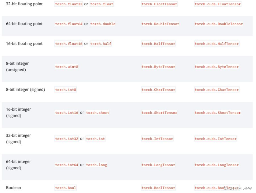
1.张量的数据类型
PyTorch有9种CPU张量类型和9种GPU张量类型:
2.张量基本信息
tensor = torch.randn(3,4,5)
print(tensor.type())  # 数据类型
print(tensor.size())  # 张量的shape,是个元组
print(tensor.dim())   # 维度的数量
3.命名张量
张量命名是一个非常有用的方法,这样可以方便地使用维度的名字来做索引或其他操作,大大提高了可读性、易用性,防止出错。
# 在PyTorch 1.3之前,需要使用注释
# Tensor[N, C, H, W]
images = torch.randn(32, 3, 56, 56)
images.sum(dim=1)
images.select(dim=1, index=0)

# PyTorch 1.3之后
NCHW = [‘N’, ‘C’, ‘H’, ‘W’]
images = torch.randn(32, 3, 56, 56, names=NCHW)
images.sum('C')
images.select('C', index=0)
# 也可以这么设置
tensor = torch.rand(3,4,1,2,names=('C', 'N', 'H', 'W'))
# 使用align_to可以对维度方便地排序
tensor = tensor.align_to('N', 'C', 'H', 'W')
4.数据类型转换
# 设置默认类型,pytorch中的FloatTensor远远快于DoubleTensor
torch.set_default_tensor_type(torch.FloatTensor)

# 类型转换
tensor = tensor.cuda()
tensor = tensor.cpu()
tensor = tensor.float()
tensor = tensor.long()
5.张量形变
# 在将卷积层输入全连接层的情况下通常需要对张量做形变处理,
# 相比torch.view,torch.reshape可以自动处理输入张量不连续的情况。
tensor = torch.rand(2,3,4)
shape = (6, 4)
tensor = torch.reshape(tensor, shape)
6.打乱顺序
tensor = tensor[torch.randperm(tensor.size(0))] # 打乱第一个维度7.复制张量
# Operation                 |  New/Shared memory | Still in computation graph |
tensor.clone()            # |        New         |          Yes               |
tensor.detach()           # |      Shared        |          No                |
tensor.detach.clone()()   # |        New         |          No                |
三、模型定义和操作
1.一个简单两层卷积网络的示例
# convolutional neural network (2 convolutional layers)
class ConvNet(nn.Module):
    def __init__(self, num_classes=10):
        super(ConvNet, self).__init__()
        self.layer1 = nn.Sequential(
            nn.Conv2d(1, 16, kernel_size=5, stride=1, padding=2),
            nn.BatchNorm2d(16),
            nn.ReLU(),
            nn.MaxPool2d(kernel_size=2, stride=2))
        self.layer2 = nn.Sequential(
            nn.Conv2d(16, 32, kernel_size=5, stride=1, padding=2),
            nn.BatchNorm2d(32),
            nn.ReLU(),
            nn.MaxPool2d(kernel_size=2, stride=2))
        self.fc = nn.Linear(7*7*32, num_classes)

    def forward(self, x):
        out = self.layer1(x)
        out = self.layer2(out)
        out = out.reshape(out.size(0), -1)
        out = self.fc(out)
        return out

model = ConvNet(num_classes).to(device)
2.双线性汇合(bilinear pooling)
X = torch.reshape(N, D, H * W)                        # Assume X has shape N*D*H*W
X = torch.bmm(X, torch.transpose(X, 1, 2)) / (H * W)  # Bilinear pooling
assert X.size() == (N, D, D)
X = torch.reshape(X, (N, D * D))
X = torch.sign(X) * torch.sqrt(torch.abs(X) + 1e-5)   # Signed-sqrt normalization
X = torch.nn.functional.normalize(X)                  # L2 normalization
3.多卡同步 BN(Batch normalization)
当使用 torch.nn.DataParallel 将代码运行在多张 GPU 卡上时,PyTorch 的 BN 层默认操作是各卡上数据独立地计算均值和标准差,同步 BN 使用所有卡上的数据一起计算 BN 层的均值和标准差,缓解了当批量大小(batch size)比较小时对均值和标准差估计不准的情况,是在目标检测等任务中一个有效的提升性能的技巧。
sync_bn = torch.nn.SyncBatchNorm(num_features, eps=1e-05, momentum=0.1, affine=True,
                                 track_running_stats=True)
4.将已有网络的所有BN层改为同步BN层
def convertBNtoSyncBN(module, process_group=None):
    '''Recursively replace all BN layers to SyncBN layer.

    Args:
        module[torch.nn.Module]. Network
    '''
    if isinstance(module, torch.nn.modules.batchnorm._BatchNorm):
        sync_bn = torch.nn.SyncBatchNorm(module.num_features, module.eps, module.momentum,
                                         module.affine, module.track_running_stats, process_group)
        sync_bn.running_mean = module.running_mean
        sync_bn.running_var = module.running_var
        if module.affine:
            sync_bn.weight = module.weight.clone().detach()
            sync_bn.bias = module.bias.clone().detach()
        return sync_bn
    else:
        for name, child_module in module.named_children():
            setattr(module, name) = convert_syncbn_model(child_module, process_group=process_group))
        return module
affine定义了BN层的参数γ和β是否是可学习的(不可学习默认是常数1和0)。
5.类似 BN 滑动平均
如果要实现类似 BN 滑动平均的操作,在 forward 函数中要使用原地(inplace)操作给滑动平均赋值。
class BN(torch.nn.Module)
    def __init__(self):
        ...
        self.register_buffer('running_mean', torch.zeros(num_features))

    def forward(self, X):
        ...
        self.running_mean += momentum * (current - self.running_mean)
6.查看网络中的参数
可以通过model.state_dict()或者model.named_parameters()函数查看现在的全部可训练参数(包括通过继承得到的父类中的参数)
params = list(model.named_parameters())
(name, param) = params[28]
print(name)
print(param.grad)
print('-------------------------------------------------')
(name2, param2) = params[29]
print(name2)
print(param2.grad)
print('----------------------------------------------------')
(name1, param1) = params[30]
print(name1)
print(param1.grad)
7.模型权重初始化
注意 model.modules() 和 model.children() 的区别:model.modules() 会迭代地遍历模型的所有子层,而 model.children() 只会遍历模型下的一层。
# Common practise for initialization.
for layer in model.modules():
    if isinstance(layer, torch.nn.Conv2d):
        torch.nn.init.kaiming_normal_(layer.weight, mode='fan_out',
                                      nonlinearity='relu')
        if layer.bias is not None:
            torch.nn.init.constant_(layer.bias, val=0.0)
    elif isinstance(layer, torch.nn.BatchNorm2d):
        torch.nn.init.constant_(layer.weight, val=1.0)
        torch.nn.init.constant_(layer.bias, val=0.0)
    elif isinstance(layer, torch.nn.Linear):
        torch.nn.init.xavier_normal_(layer.weight)
        if layer.bias is not None:
            torch.nn.init.constant_(layer.bias, val=0.0)

# Initialization with given tensor.
layer.weight = torch.nn.Parameter(tensor)
四、数据处理
1.计算数据集的均值和标准差
import os
import cv2
import numpy as np
from torch.utils.data import Dataset
from PIL import Image


def compute_mean_and_std(dataset):
    # 输入PyTorch的dataset,输出均值和标准差
    mean_r = 0
    mean_g = 0
    mean_b = 0

    for img, _ in dataset:
        img = np.asarray(img) # change PIL Image to numpy array
        mean_b += np.mean(img[:, :, 0])
        mean_g += np.mean(img[:, :, 1])
        mean_r += np.mean(img[:, :, 2])

    mean_b /= len(dataset)
    mean_g /= len(dataset)
    mean_r /= len(dataset)

    diff_r = 0
    diff_g = 0
    diff_b = 0

    N = 0

    for img, _ in dataset:
        img = np.asarray(img)

        diff_b += np.sum(np.power(img[:, :, 0] - mean_b, 2))
        diff_g += np.sum(np.power(img[:, :, 1] - mean_g, 2))
        diff_r += np.sum(np.power(img[:, :, 2] - mean_r, 2))

        N += np.prod(img[:, :, 0].shape)

    std_b = np.sqrt(diff_b / N)
    std_g = np.sqrt(diff_g / N)
    std_r = np.sqrt(diff_r / N)

    mean = (mean_b.item() / 255.0, mean_g.item() / 255.0, mean_r.item() / 255.0)
    std = (std_b.item() / 255.0, std_g.item() / 255.0, std_r.item() / 255.0)
    return mean, std
2.常用训练和验证数据预处理
其中 ToTensor 操作会将 PIL.Image 或形状为 H×W×D,数值范围为 [0, 255] 的 np.ndarray 转换为形状为 D×H×W,数值范围为 [0.0, 1.0] 的 torch.Tensor。
train_transform = torchvision.transforms.Compose([
    torchvision.transforms.RandomResizedCrop(size=224,
                                             scale=(0.08, 1.0)),
    torchvision.transforms.RandomHorizontalFlip(),
    torchvision.transforms.ToTensor(),
    torchvision.transforms.Normalize(mean=(0.485, 0.456, 0.406),
                                     std=(0.229, 0.224, 0.225)),
 ])
 val_transform = torchvision.transforms.Compose([
    torchvision.transforms.Resize(256),
    torchvision.transforms.CenterCrop(224),
    torchvision.transforms.ToTensor(),
    torchvision.transforms.Normalize(mean=(0.485, 0.456, 0.406),
                                     std=(0.229, 0.224, 0.225)),
])
五、模型训练和测试
1.分类模型训练代码
# Loss and optimizer
criterion = nn.CrossEntropyLoss()
optimizer = torch.optim.Adam(model.parameters(), lr=learning_rate)

# Train the model
total_step = len(train_loader)
for epoch in range(num_epochs):
    for i ,(images, labels) in enumerate(train_loader):
        images = images.to(device)
        labels = labels.to(device)

        # Forward pass
        outputs = model(images)
        loss = criterion(outputs, labels)

        # Backward and optimizer
        optimizer.zero_grad()
        loss.backward()
        optimizer.step()

        if (i+1) % 100 == 0:
            print('Epoch: [{}/{}], Step: [{}/{}], Loss: {}'
                  .format(epoch+1, num_epochs, i+1, total_step, loss.item()))
2.分类模型测试代码
# Test the model
model.eval()  # eval mode(batch norm uses moving mean/variance
              #instead of mini-batch mean/variance)
with torch.no_grad():
    correct = 0
    total = 0
    for images, labels in test_loader:
        images = images.to(device)
        labels = labels.to(device)
        outputs = model(images)
        _, predicted = torch.max(outputs.data, 1)
        total += labels.size(0)
        correct += (predicted == labels).sum().item()

    print('Test accuracy of the model on the 10000 test images: {} %'
          .format(100 * correct / total))
3.自定义loss
继承torch.nn.Module类写自己的loss。
class MyLoss(torch.nn.Module):
    def __init__(self):
        super(MyLoss, self).__init__()

    def forward(self, x, y):
        loss = torch.mean((x - y) ** 2)
        return loss
4.标签平滑(label smoothing)
写一个label_smoothing.py的文件,然后在训练代码里引用,用LSR代替交叉熵损失即可。label_smoothing.py内容如下:
import torch
import torch.nn as nn


class LSR(nn.Module):

    def __init__(self, e=0.1, reduction='mean'):
        super().__init__()

        self.log_softmax = nn.LogSoftmax(dim=1)
        self.e = e
        self.reduction = reduction

    def _one_hot(self, labels, classes, value=1):
        """
            Convert labels to one hot vectors

        Args:
            labels: torch tensor in format [label1, label2, label3, ...]
            classes: int, number of classes
            value: label value in one hot vector, default to 1

        Returns:
            return one hot format labels in shape [batchsize, classes]
        """

        one_hot = torch.zeros(labels.size(0), classes)

        #labels and value_added  size must match
        labels = labels.view(labels.size(0), -1)
        value_added = torch.Tensor(labels.size(0), 1).fill_(value)

        value_added = value_added.to(labels.device)
        one_hot = one_hot.to(labels.device)

        one_hot.scatter_add_(1, labels, value_added)

        return one_hot

    def _smooth_label(self, target, length, smooth_factor):
        """convert targets to one-hot format, and smooth
        them.
        Args:
            target: target in form with [label1, label2, label_batchsize]
            length: length of one-hot format(number of classes)
            smooth_factor: smooth factor for label smooth

        Returns:
            smoothed labels in one hot format
        """
        one_hot = self._one_hot(target, length, value=1 - smooth_factor)
        one_hot += smooth_factor / (length - 1)

        return one_hot.to(target.device)

    def forward(self, x, target):

        if x.size(0) != target.size(0):
            raise ValueError('Expected input batchsize ({}) to match target batch_size({})'
                    .format(x.size(0), target.size(0)))

        if x.dim() < 2:
            raise ValueError('Expected input tensor to have least 2 dimensions(got {})'
                    .format(x.size(0)))

        if x.dim() != 2:
            raise ValueError('Only 2 dimension tensor are implemented, (got {})'
                    .format(x.size()))


        smoothed_target = self._smooth_label(target, x.size(1), self.e)
        x = self.log_softmax(x)
        loss = torch.sum(- x * smoothed_target, dim=1)

        if self.reduction == 'none':
            return loss

        elif self.reduction == 'sum':
            return torch.sum(loss)

        elif self.reduction == 'mean':
            return torch.mean(loss)

        else:
            raise ValueError('unrecognized option, expect reduction to be one of none, mean, sum')
5.模型训练可视化
PyTorch可以使用tensorboard来可视化训练过程。
安装和运行TensorBoard。
pip install tensorboard
tensorboard --logdir=runs
使用SummaryWriter类来收集和可视化相应的数据,放了方便查看,可以使用不同的文件夹,比如'Loss/train'和'Loss/test'。
from torch.utils.tensorboard import SummaryWriter
import numpy as np

writer = SummaryWriter()

for n_iter in range(100):
    writer.add_scalar('Loss/train', np.random.random(), n_iter)
    writer.add_scalar('Loss/test', np.random.random(), n_iter)
    writer.add_scalar('Accuracy/train', np.random.random(), n_iter)
    writer.add_scalar('Accuracy/test', np.random.random(), n_iter)
6.保存与加载断点
注意为了能够恢复训练,我们需要同时保存模型和优化器的状态,以及当前的训练轮数。
start_epoch = 0
# Load checkpoint.
if resume: # resume为参数,第一次训练时设为0,中断再训练时设为1
    model_path = os.path.join('model', 'best_checkpoint.pth.tar')
    assert os.path.isfile(model_path)
    checkpoint = torch.load(model_path)
    best_acc = checkpoint['best_acc']
    start_epoch = checkpoint['epoch']
    model.load_state_dict(checkpoint['model'])
    optimizer.load_state_dict(checkpoint['optimizer'])
    print('Load checkpoint at epoch {}.'.format(start_epoch))
    print('Best accuracy so far {}.'.format(best_acc))

# Train the model
for epoch in range(start_epoch, num_epochs):
    ...

    # Test the model
    ...

    # save checkpoint
    is_best = current_acc > best_acc
    best_acc = max(current_acc, best_acc)
    checkpoint = {
        'best_acc': best_acc,
        'epoch': epoch + 1,
        'model': model.state_dict(),
        'optimizer': optimizer.state_dict(),
    }
    model_path = os.path.join('model', 'checkpoint.pth.tar')
    best_model_path = os.path.join('model', 'best_checkpoint.pth.tar')
    torch.save(checkpoint, model_path)
    if is_best:
        shutil.copy(model_path, best_model_path)
六、其他注意事项
-
不要使用太大的线性层。因为nn.Linear(m,n)使用的是O(m,n)的内存,线性层太大很容易超出现有显存。
-
不要在太长的序列上使用RNN。因为RNN反向传播使用的是BPTT算法,其需要的内存和输入序列的长度呈线性关系。
-
model(x) 前用 model.train() 和 model.eval() 切换网络状态。
-
不需要计算梯度的代码块用 with torch.no_grad() 包含起来。
-
model.eval() 和 torch.no_grad() 的区别在于,model.eval() 是将网络切换为测试状态,例如 BN 和dropout在训练和测试阶段使用不同的计算方法。torch.no_grad() 是关闭 PyTorch 张量的自动求导机制,以减少存储使用和加速计算,得到的结果无法进行 loss.backward()。
-
model.zero_grad()会把整个模型的参数的梯度都归零, 而optimizer.zero_grad()只会把传入其中的参数的梯度归零。
-
torch.nn.CrossEntropyLoss 的输入不需要经过 Softmax。torch.nn.CrossEntropyLoss 等价于 torch.nn.functional.log_softmax + torch.nn.NLLLoss。
-
loss.backward() 前用 optimizer.zero_grad() 清除累积梯度。
-
torch.utils.data.DataLoader 中尽量设置 pin_memory=True,对特别小的数据集如 MNIST 设置 pin_memory=False 反而更快一些。num_workers 的设置需要在实验中找到最快的取值。
-
用 del 及时删除不用的中间变量,节约 GPU 存储。
-
减少 CPU 和 GPU 之间的数据传输。 例如如果你想知道一个 epoch 中每个 mini-batch 的 loss 和准确率,先将它们累积在 GPU 中等一个 epoch 结束之后一起传输回 CPU 会比每个 mini-batch 都进行一次 GPU 到 CPU 的传输更快。
-
使用半精度浮点数 half() 会有一定的速度提升,具体效率依赖于 GPU 型号。需要小心数值精度过低带来的稳定性问题。
-
时常使用 assert tensor.size() == (N, D, H, W) 作为调试手段,确保张量维度和你设想中一致。
-
除了标记 y 外,尽量少使用一维张量,使用 n*1 的二维张量代替,可以避免一些意想不到的一维张量计算结果。