主动学习ALEC算法——Java之旅

概述

  ALEC的概念我们已经说过啦，需要了解的同学请点击这里。在旅行出发之前我们来看看这次旅行的生活用品，看看这个算法中的主要成员变量。注意不要死记，结合我们在概念中讲的原理理解记忆。完整代码点击这里，建议先看概念抓住逻辑框架，再一遍代码注释形成初步理解，再看此文会理解更深。

成员变量

public class Alec {
    
    
	/**
	 * 整个数据集
	 */
	Instances dataset;

	/**
	 * 可以提供的最大查询数。
	 */
	int maxNumQuery;

	/**
	 * 查询的实际数量。
	 */
	int numQuery;

	/**
	 * 半径, 也是论文的dc. 它用于密度计算。
	 */
	double radius;

	/**
	 * 实例的密度, 论文中的rho.
	 */
	double[] densities;

	/**
	 * 到老大之间的距离
	 */
	double[] distanceToMaster;

	/**
	 * 给索引排序, 其中第一个元素表示密度最大的实例。
	 * 
	 */
	int[] descendantDensities;

	/**
	 * 优先级
	 */
	double[] priority;

	/**
	 * 任意两点之间的最大距离。
	 */
	double maximalDistance;

	/**
	 * 上级，大哥
	 */
	int[] masters;

	/**
	 * 预测标签
	 */
	int[] predictedLabels;

	/**
	 * 实例状态。0表示未处理，1表示已查询，2表示已分类。
	 */
	int[] instanceStatusArray;

	/**
	 * 子代索引以子代顺序显示实例的代表性。
	 * 
	 */
	int[] descendantRepresentatives;

	/**
	 * 指出每个实例的集群. 它仅被用于clusterInTwo(int[]);
	 */
	int[] clusterIndices;

	/**
	 * 大小不超过此阈值的块不应进一步拆分。
	 */
	int smallBlockThreshold = 3;

主函数(程序入口)

  各位旅客同志们请拿好自己的行李，请到检票口进行检票，我们即将发车。

	public static void main(String[] args) {
    
    
		long tempStart = System.currentTimeMillis();

		System.out.println("Starting ALEC.");
		String arffFilename = "D:/data/iris.arff";
		// String arffFilename = "D:/data/mushroom.arff";

		Alec tempAlec = new Alec(arffFilename);
		// The settings for iris
		tempAlec.clusterBasedActiveLearning(0.15, 30, 3);
		// The settings for mushroom
		// tempAlec.clusterBasedActiveLearning(0.1, 800, 3);
		System.out.println(tempAlec);

		long tempEnd = System.currentTimeMillis();
		System.out.println("Runtime: " + (tempEnd - tempStart) + "ms.");
	}// Of main

  System.currentTimeMillis()，计算一段代码执行的时间，可以通过该方法获取到起始时间，结束时间，然后计算时间差，最后再进行时间单位的转换。也就是用来记录我们这班车要做多长时间。随后便是导入数据集，走，进去看看。

文件读取

	public Alec(String paraFilename) {
    
    
		try {
    
    
			FileReader tempReader = new FileReader(paraFilename);
			dataset = new Instances(tempReader);
			dataset.setClassIndex(dataset.numAttributes() - 1);
			tempReader.close();
		} catch (Exception ee) {
    
    
			System.out.println(ee);
			System.exit(0);
		} // Of fry
		computeMaximalDistance();
		clusterIndices = new int[dataset.numInstances()];// 空间变成了数据集的大小
	}// Of the constructor

  很多部分是一样的，但是看看这两句话。

		computeMaximalDistance();
		clusterIndices = new int[dataset.numInstances()];// 空间变成了数据集的大小

computeMaximalDistance（）

	public void computeMaximalDistance() {
    
    
		maximalDistance = 0;
		double tempDistance;
		for (int i = 0; i < dataset.numInstances(); i++) {
    
     // 对每一个变量进行循环，找出最大值
			for (int j = 0; j < dataset.numInstances(); j++) {
    
    
				tempDistance = distance(i, j);// 计算两点直接的距离
				if (maximalDistance < tempDistance) {
    
    
					maximalDistance = tempDistance;
				} // Of if
			} // Of for j
		} // Of for i

		System.out.println("maximalDistance = " + maximalDistance);
	}// Of computeMaximalDistance

  这里就是计算出这个数据集两个样本的之间最大的距离，计算完之后我们就打印出来，他有什么用呢？

clusterBasedActiveLearning(double paraRatio, int paraMaxNumQuer)

	public void clusterBasedActiveLearning(double paraRatio, int paraMaxNumQuery,
			int paraSmallBlockThreshold) {
    
    
		radius = maximalDistance * paraRatio; // 原来这个比例就是乘以最大的距离 表示 dc
		smallBlockThreshold = paraSmallBlockThreshold; // 一个块中的最小样本点个数

		maxNumQuery = paraMaxNumQuery; // 查询的最大个数
		predictedLabels = new int[dataset.numInstances()]; // 标签预测数组

		for (int i = 0; i < dataset.numInstances(); i++) {
    
    
			predictedLabels[i] = -1; // 对其进行初始化。
		} // Of for i

		computeDensitiesGaussian(); // 密度计算
		computeDistanceToMaster(); // 到大哥之间的距离
		computePriority(); // 优先级
		descendantRepresentatives = mergeSortToIndices(priority); // 对优先级排序，是一个降序
		System.out.println(
				"descendantRepresentatives = " + Arrays.toString(descendantRepresentatives));

		numQuery = 0;
		clusterBasedActiveLearning(descendantRepresentatives);
	}// Of clusterBasedActiveLearning

  这个方法有重载，我们先介绍第一个。这里传过来三个参数，比例，最大查询的标签数目，以及我们分块时最小的限度。来回答刚刚提出的问题，maximalDistance 的作用便是乘以这个比例 ratio 来获得我们半径。经过一轮初始化，预测标签数组值为 -1 。物以类聚人以群分，我们现在就去看看怎么去找属于我们那一类的大哥。

computeDensitiesGaussian() 方法

	public void computeDensitiesGaussian() {
    
    
		System.out.println("radius = " + radius);
		densities = new double[dataset.numInstances()];// 实例的密度数组它的大小是实例数目
		double tempDistance;

		for (int i = 0; i < dataset.numInstances(); i++) {
    
    
			for (int j = 0; j < dataset.numInstances(); j++) {
    
    
				tempDistance = distance(i, j);// 计算出两点之间的距离
				densities[i] += Math.exp(-tempDistance * tempDistance / radius / radius);
			} // Of for j
		} // Of for i

		System.out.println("The densities are " + Arrays.toString(densities) + "\r\n");
	}// Of computeDensitiesGaussian

  这个高斯密度就不得了，我们之前的 knn,k-Means 是通过距离的，高斯密度就把距离和样本数进行综合考虑。$$density=\sum _{j=1}^n{e}^{-(\frac{d^2}{r^2})}$$
什么意思，我们要计算以这个点为中心，半径 r 内的密度。我们就去对所有样本进行计算距离，然后再来看贡献度，你距离越大我们的 density 越小，贡献度越低，当距离接近 0 的时候，贡献度就是1，把所有的点贡献度加起来就得到了密度。你问我那么这个点的孩子有多少个呢？我的回答是，不知道，至少这个方法看不出来，我们只知道某点的密度最大。

computeDistanceToMaster() 找大哥

	public void computeDistanceToMaster() {
    
    
		distanceToMaster = new double[dataset.numInstances()]; // 到大哥之间的距离
		masters = new int[dataset.numInstances()]; // 大哥数组
		descendantDensities = new int[dataset.numInstances()]; // 降序排列的密度
		instanceStatusArray = new int[dataset.numInstances()]; // 状态数组

		descendantDensities = mergeSortToIndices(densities); // 对密度进行降序排列，然后返回索引
		distanceToMaster[descendantDensities[0]] = maximalDistance; // 密度最大的点没有大哥，他就是爷(根节点)

		double tempDistance;
		for (int i = 1; i < dataset.numInstances(); i++) {
    
     // 从第二高的密度点去寻找自己的老大
			// 初始化
			distanceToMaster[descendantDensities[i]] = maximalDistance; // 初始化，和大哥的距离设置为最远
			for (int j = 0; j <= i - 1; j++) {
    
     // 我们找大哥，一定要找密度比自己大的点，不然凭什么做我的大哥呢？
				tempDistance = distance(descendantDensities[i], descendantDensities[j]); // 计算距离
				if (distanceToMaster[descendantDensities[i]] > tempDistance) {
    
    
					distanceToMaster[descendantDensities[i]] = tempDistance;
					masters[descendantDensities[i]] = descendantDensities[j]; // 选择最近的距离作为我的大哥。
				} // Of if 
			} // Of for j
		} // Of for i
		System.out.println("First compute, masters = " + Arrays.toString(masters));
		System.out.println("descendantDensities = " + Arrays.toString(descendantDensities));
	}// Of computeDistanceToMaster

  每句话的分析已经列上，我们找大哥是由要求的：第一你的密度要比我的大，第二距离还要最近，远亲不如近邻嘛。

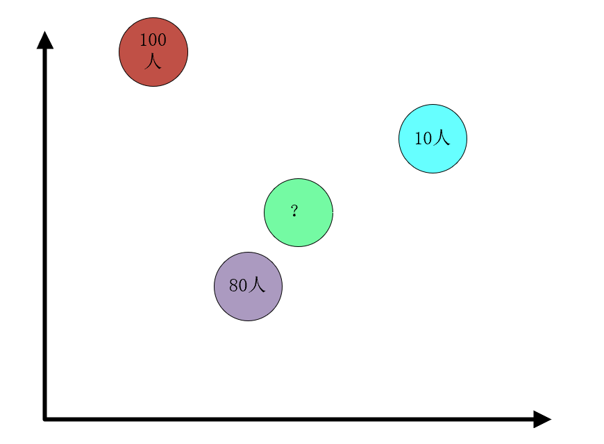
绿球找谁做大哥？100人的褐色球太远，起冲突了等你人过来黄花菜都凉了，10太少了，综合考虑人数距离我们选择和紫色球搞好关系，认他做大哥。接下来我们要做的便是给大哥排序，返回大哥的住址，而不是密度大小哦！这里有一点绕，我们才一点刹车慢慢来看。

mergeSortToIndices(densities) 给大哥排序

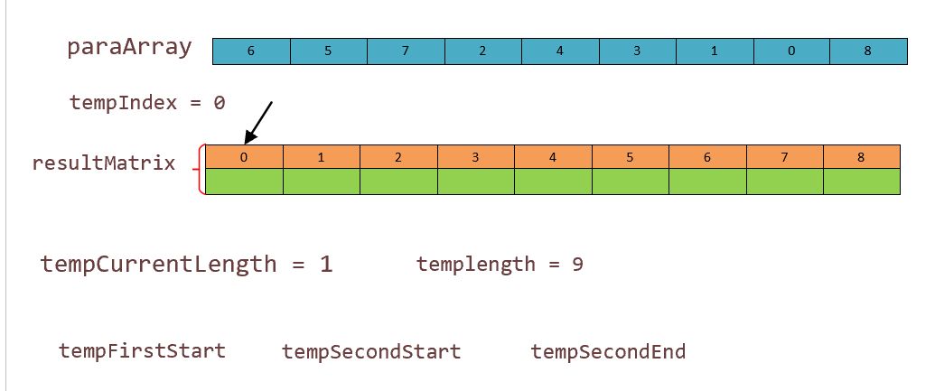
public static int[] mergeSortToIndices(double[] paraArray) {
    
    
		int tempLength = paraArray.length;
		int[][] resultMatrix = new int[2][tempLength];// 用于归并排序，两个数组来回跳跃。

		// 初始化
		int tempIndex = 0;
		for (int i = 0; i < tempLength; i++) {
    
    
			resultMatrix[tempIndex][i] = i;
		} // Of for i

		// 归并
		int tempCurrentLength = 1;
		// 当前合并组的索引。
		int tempFirstStart, tempSecondStart, tempSecondEnd;

		while (tempCurrentLength < tempLength) {
    
    
			// 分成两组
			// 这里的边界自适应于不等于2^k的数组长度。math.ceil(x)返回大于等于参数x的最小整数,即对浮点数向上取整.
			for (int i = 0; i < Math.ceil((tempLength + 0.0) / tempCurrentLength / 2); i++) {
    
    
				// 块的界限
				tempFirstStart = i * tempCurrentLength * 2;

				tempSecondStart = tempFirstStart + tempCurrentLength;

				tempSecondEnd = tempSecondStart + tempCurrentLength - 1;
				if (tempSecondEnd >= tempLength) {
    
    
					tempSecondEnd = tempLength - 1;
				} // Of if

				// 对这个组进行归并
				int tempFirstIndex = tempFirstStart;
				int tempSecondIndex = tempSecondStart;
				int tempCurrentIndex = tempFirstStart;

				if (tempSecondStart >= tempLength) {
    
    
					for (int j = tempFirstIndex; j < tempLength; j++) {
    
    
						resultMatrix[(tempIndex + 1) % 2][tempCurrentIndex] = resultMatrix[tempIndex
								% 2][j];
						tempFirstIndex++;
						tempCurrentIndex++;
					} // Of for j
					break;
				} // Of if

				while ((tempFirstIndex <= tempSecondStart - 1)
						&& (tempSecondIndex <= tempSecondEnd)) {
    
    

					if (paraArray[resultMatrix[tempIndex
							% 2][tempFirstIndex]] >= paraArray[resultMatrix[tempIndex
									% 2][tempSecondIndex]]) {
    
    
						resultMatrix[(tempIndex + 1) % 2][tempCurrentIndex] = resultMatrix[tempIndex
								% 2][tempFirstIndex];
						tempFirstIndex++;
					} else {
    
    
						resultMatrix[(tempIndex + 1) % 2][tempCurrentIndex] = resultMatrix[tempIndex
								% 2][tempSecondIndex];
						tempSecondIndex++;
					} // Of if
					tempCurrentIndex++;
				} // Of while

				// 剩余部分。
				for (int j = tempFirstIndex; j < tempSecondStart; j++) {
    
    
					resultMatrix[(tempIndex + 1) % 2][tempCurrentIndex] = resultMatrix[tempIndex
							% 2][j];
					tempCurrentIndex++;
				} // Of for j
				for (int j = tempSecondIndex; j <= tempSecondEnd; j++) {
    
    
					resultMatrix[(tempIndex + 1) % 2][tempCurrentIndex] = resultMatrix[tempIndex
							% 2][j];
					tempCurrentIndex++;
				} // Of for j
			} // Of for i

			tempCurrentLength *= 2;
			tempIndex++;
		} // Of while

		return resultMatrix[tempIndex % 2];
	}// Of mergeSortToIndices

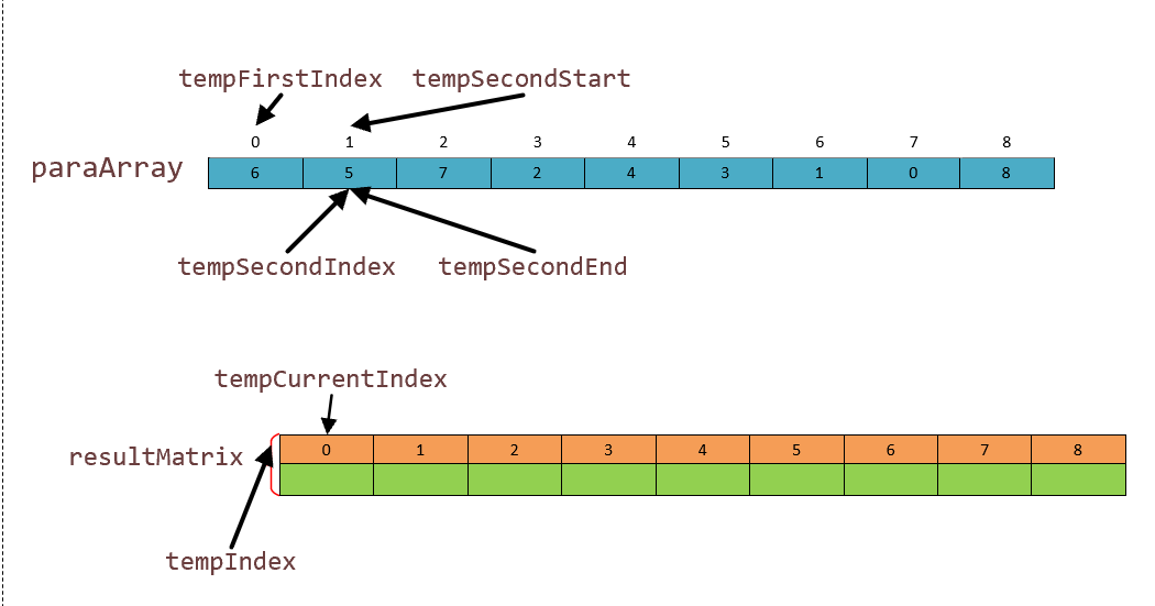
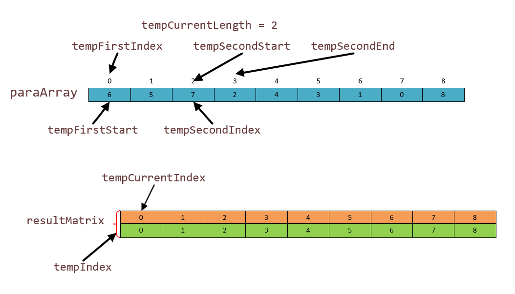
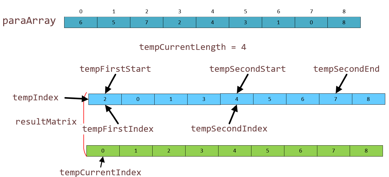
  这个地方是一个难点，我们将细致一点。首先程序运行到第一个 while 我们对一些变量初始化如图：

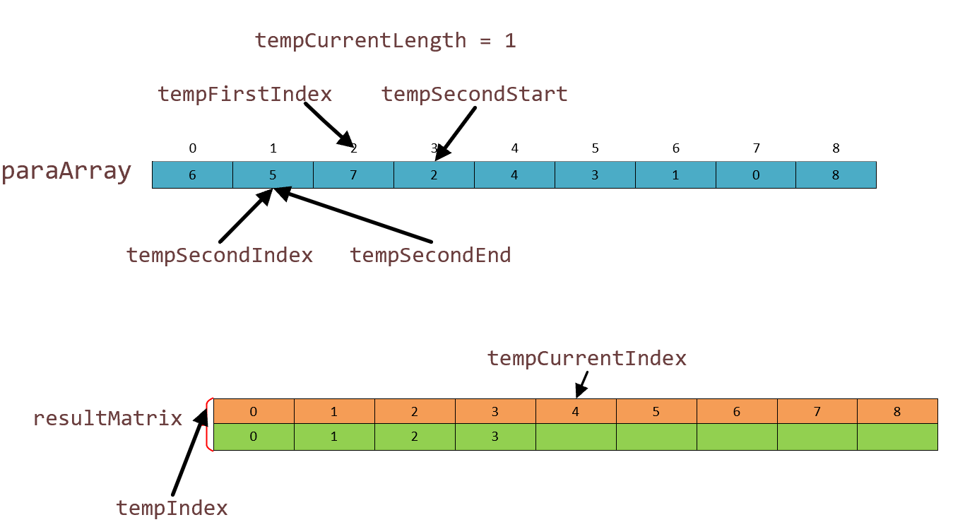
之后我们遍进入第一个 while 进行 for 循环分块，第一次，终止条件 i = 5. 按照程序初始话 tempFirstStart,tempSecondStart,tempSecondEnd 赋值如图：

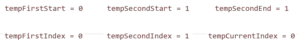
if (tempSecondStart >= tempLength)

因为 1 < 9,所以我们这里的不会执行里面的 for 循环 ，直接转入第二 while 。第二个 while 就是进行比较，在这里我们先来看一看比较的原理：

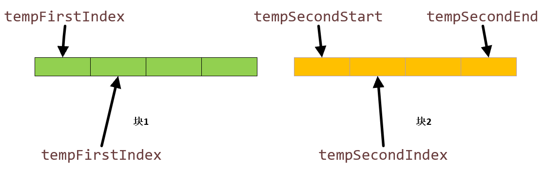
我们比较是两个子块的大小，tempFirstStart,tempSecondStart,tempSecondEnd 用来卡主两个块的位置，即开始点和结束比较点。而tempIndex 和 tempSecondIndex 在这两个块中移动，用他们两个所指向的元素比较大小，排序。我们第二 while 循环范围便是前面两个元素进行比较。如图：

我们把 paraArray 里面前两个数进行比较，发现 6 > 5,然后我们把对应的索引进行交换放在第绿色的那一列。

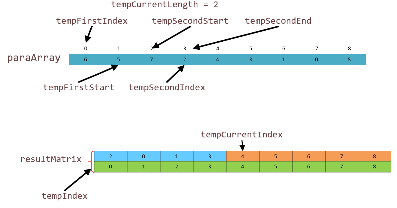
我们进行第二轮：两两比较，该比较 2 和 3 位置的元素。这里我可以解释一下：tempCurrentLength 就是控制两个块的大小，tempCurrentIndex 负责我们索引数组的移动。 ，我们这里是1，所以tempFirst哪些卡位指针集体往右移动去寻找未排序的范围，这里从 [0] [1] 跑到了 [2] [3].如图：

  在这里跳过一次，来看看最后剩一个 8 怎么处理 ？再来看看代码

tempSecondStart = tempFirstStart + tempCurrentLength; // 从第一块的第一个开始，+ 长度就会到达第二个开始点

				tempSecondEnd = tempSecondStart + tempCurrentLength - 1; // 记录第二块结束位置，第二块开始+长度-1
				if (tempSecondEnd >= tempLength) {
    
     // 如果第二次end 长度超过了数组的长度,下面一句进行回退。
					tempSecondEnd = tempLength - 1; 
				} // Of if

				// 对这个组进行归并，把开始的两个引用，复制给两次开始的索引，tempcurrentIndex也是第一次开始的引用
				int tempFirstIndex = tempFirstStart; 
				int tempSecondIndex = tempSecondStart;
				int tempCurrentIndex = tempFirstStart;

				if (tempSecondStart >= tempLength) {
    
     // 如果第二部分开始的引用大于块长度
					for (int j = tempFirstIndex; j < tempLength; j++) {
    
     // 就从第一个块开始，遍历
						resultMatrix[(tempIndex + 1) % 2][tempCurrentIndex] = resultMatrix[tempIndex
								% 2][j]; // 把数组填满。
						tempFirstIndex++;
						tempCurrentIndex++;
					} // Of for j
					break;
				} // Of if

最后一个指针是这样子的

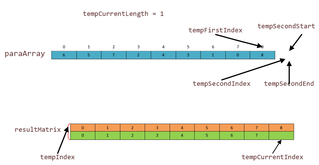
注意看啊，tempSecondStart 和 tempSecondEnd tempSecondIndex 指向 9 越界了，然后我们用一个 if 语句来判断，越界？那我就把 tempSecondEnd 拉回 8 的位置，然后进行赋值。但是，我们要注意，tempSecondIndex 的值来自于tempSecondStart,所以是 9 。也就是说我们第二个块开始就不存在，为空了。然后我们再来一个 if 对第二个块为空的情况处理，便是把块1的值赋值到索引数组中去。

			tempCurrentLength *= 2;
			tempIndex++;

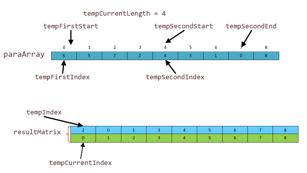
长度翻倍，现在我们就把索引第一个位置作为结果储存去了。状况如图：

现在我们再来比较，当块的长度是2时，第一轮比较：0 号位和 2 号位比较，6 < 7,7号元素进入resultMatrix数组[0] [0],tempCuurentIndex控制着结果存放位置，指针后移一个。第二块的遍历指针 tempSecondIndex 后移一位与 6 比较，发现 6 大，那么 0 号索引进入索引数组 resultMatrix [0][1]结果如下图：

resultMatrix中蓝色的部分就是我们这一轮排好的索引。接下来我们对后面4个进行归并排序，操作流程一样我们不在描述了。然后只剩一个块，操作和 tempCurrentLength = 1,剩一个块的情况一模一样，不在赘述了，列出第二轮结果图(8 号元素没有轮到，其实最后一步也是直接复制进去)：

这时候 tempCurrentLength 变成 4 了，块的大小变成了 4。现在我们进行比较，你说会这不都一样吗？但是没有私货怎么敢写呢，这里主要给大家说说明明我们 tempArray 数组没有改变，改变的是储存数组，既然 tempArray 数组都没有改变，怎么叫排序呢，这不是胡扯嘛。听我细细说来：先交代一下，tempMatrix 储存结果换到了第二行。初始值指针如下

排序核心寻址

verygood，如果你现在比较的话是按照 tempArray 这个顺序的话，那你就等于没有排序，实际上是需要我们 resultMatrix 数组的第一行作为参考去寻址，第一个位置储存的不是6 ，而是 2 号位置的 7。也就是说我们把 tempMattrix 数组的蓝色空间储存的地址，按照 tempArray 数组还原成这样，对这个数组进行归并的。

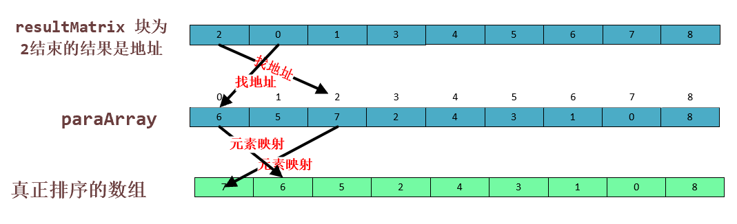
注意第三个数组是虚拟的，我们便于直观画出来的 下面便是处理这中行为的代码：也就是比较部分

				while ((tempFirstIndex <= tempSecondStart - 1)// 如果第一个块的位置，没有和第二个块开始的位置衔接，
						&& (tempSecondIndex <= tempSecondEnd)) {
    
     // 第二个块开始的位置没有和第二个块结束的位置衔接，那么执行迭代 

					if (paraArray[resultMatrix[tempIndex% 2][tempFirstIndex]] >= paraArray[resultMatrix[tempIndex% 2][tempSecondIndex]]) {
    
    
						resultMatrix[(tempIndex + 1) % 2][tempCurrentIndex] = resultMatrix[tempIndex% 2][tempFirstIndex];
						tempFirstIndex++;
					} else {
    
    
						resultMatrix[(tempIndex + 1) % 2][tempCurrentIndex] = resultMatrix[tempIndex% 2][tempSecondIndex];
						tempSecondIndex++; // 比较数组指针移动
					} // Of if
					tempCurrentIndex++; // 索引数组指针移动
				} // Of while

那么我就可以纠正一下 我上面的错误了，为了方便理解，我直接把tempFirst,等一系列指针画在了 tempArray 数组中，实际上它是在 tempMatrix 数组中进行卡范围，遍历游走，tempArray 数组只是作为一个映射标准，没有动用它。真实情况如图：

重复昨天的故事，知道排序完成。呀呼~，返回一个排序好的数组索引：8, 2, 0, 1, 4, 5, 3, 6, 7
小结：

1. tempFirstStart,tempSecondStart,tempSecondEnd 用来卡主两个块的位置
2. tempFirstIndex,tempSecondIndex负责在这两个块中遍历比较，实际最多只有两个块的比较大小排序
3. tempCurrentLength 负责控制块的大小
4. tempCurrentIndex 负责控制 tempMatrix 数组存储位置，元素放进来一个后移一位
5. tempMatrix 数组是一个二维数组，我把空间分成： 排序参照地址区 和 存储结果区，上面 1,2两点索引都在 排序参照地址区。排序参照地址区 开始阶段是参考 tempArray 数组初始化地址，其后的更新都是每一轮 tempCurrentLength = n 局部排序完成的结果。
6. tempIndex 是负责 排序参照区 和 存储结果区 互换的指针，我们把排好序的结果逐个放在排序参照区，那么正在使用的 排序参照区 将会慢慢变为 存储结果区，而排序完成后，这个 排序参照区 转化成了 存储结果区，下一轮开始又会成为下一轮的参照区。另外一个区对立转化
7. 总的思路：一个地址映射数组 tempArray数组，地址索引数组 tempMatrix[][].归并排序是两个块开始为 1，同步移动的两个块，当块中的元素变多，当一个块完成比较，另外一个块的剩下序号有序可以直接复制进去。如果最后一个单着的元素，将会一直单着，知道最后一次归并纳入排序。

  花了大量的时间来解释这个排序返回地址的方法，是因为这在机器学习的处理中很常用，要搞懂，当然你要用Python那就另当别论了哈哈哈。下面我们继续旅途，刚刚爬了一座山有没有累?出去走一下吧，后面的内容将会轻松许多。

descendantDensities = mergeSortToIndices(densities);

第266行，我们在这里获得了一个降序排列的索引密度数组，第 267 行就是把这个密度数组的最大密度设置成大哥。270~283就是在密度数组中来选取大哥，一定记得在比自己高的密度结点中选取距离近的哦。
  这里就完成了优先级的排序，大哥的选择。下面我们将进入基于主动学习的聚类了，这里也是核心但是没有那么绕了，这个方法是重载的。

clusterBasedActiveLearning(descendantRepresentatives)

	public void clusterBasedActiveLearning(int[] paraBlock) {
    
    
		System.out.println("clusterBasedActiveLearning for block " + Arrays.toString(paraBlock));

		// Step 1. 这个块可以查询的最大长度
		int tempExpectedQueries = (int) Math.sqrt(paraBlock.length); // 这个块可以查询的最大长度
		int tempNumQuery = 0;
		for (int i = 0; i < paraBlock.length; i++) {
    
    // 统计查询过的数量
			if (instanceStatusArray[paraBlock[i]] == 1) {
    
    
				tempNumQuery++;
			} // Of if
		} // Of for i

		// Step 2. 如果我们的查询数量超过预期用完了，这个块的数目小于最小块我们进行投票。
		if ((tempNumQuery >= tempExpectedQueries) && (paraBlock.length <= smallBlockThreshold)) {
    
    
			System.out.println("" + tempNumQuery + " instances are queried, vote for block: \r\n"
					+ Arrays.toString(paraBlock));
			vote(paraBlock);

			return;
		} // Of if

		// Step 3. Query enough labels.
		for (int i = 0; i < tempExpectedQueries; i++) {
    
    
			if (numQuery >= maxNumQuery) {
    
    
				System.out.println("No more queries are provided, numQuery = " + numQuery + ".");
				vote(paraBlock);
				return;
			} // Of if

			if (instanceStatusArray[paraBlock[i]] == 0) {
    
    
				instanceStatusArray[paraBlock[i]] = 1;
				predictedLabels[paraBlock[i]] = (int) dataset.instance(paraBlock[i]).classValue();
				// System.out.println("Query #" + paraBlock[i] + ", numQuery = "
				// + numQuery);
				numQuery++;
			} // Of if
		} // Of for i

		// Step 4. Pure?
		int tempFirstLabel = predictedLabels[paraBlock[0]];
		boolean tempPure = true;
		for (int i = 1; i < tempExpectedQueries; i++) {
    
    
			if (predictedLabels[paraBlock[i]] != tempFirstLabel) {
    
    
				tempPure = false;
				break;
			} // Of if
		} // Of for i
		if (tempPure) {
    
    
			System.out.println("Classify for pure block: " + Arrays.toString(paraBlock));
			for (int i = tempExpectedQueries; i < paraBlock.length; i++) {
    
    
				if (instanceStatusArray[paraBlock[i]] == 0) {
    
    
					predictedLabels[paraBlock[i]] = tempFirstLabel;
					instanceStatusArray[paraBlock[i]] = 2;
				} // Of if
			} // Of for i
			return;
		} // Of if

		// Step 5. Split in two and process them independently.
		int[][] tempBlocks = clusterInTwo(paraBlock);
		for (int i = 0; i < 2; i++) {
    
    
			// Attention: recursive invoking here.
			clusterBasedActiveLearning(tempBlocks[i]);
		} // Of for i
	}// Of clusterBasedActiveLearning

1. 459 - 475 行设置这个块的最大查询数目，然后看看这个块已经查询了多少标签，查询数目上限，又是小块(小于一个块最小的域值)。我们进行投票判断这个块的种类。
2. 478 - 492一个 for 循环去查询更多的标签，如果查询的数目已经大于了总的查询数目，我们进行投票决定这个块的类别。反之我们就会查询这个块的高密度实例。
3. 495 - 502 行判断我们这个块是否为纯的：这个块的第一个实例密度最高，它的类本应该代表它后面的实例，因此我们把其后面查询的标签和老大比较，相同则纯，反之由杂。
4. 503 - 520 行，如果块是纯的，那么我们就给这个块没有查询的实例贴上和老大一样的类 tempFirstlable ,查询状态值为2( 2 代表是学习器判断的标签，0 代表未知种类，1 代表向教授查询的标签)。如果不纯，那么我们继续分块咯，你不服从那就自立家门吧，重复以上操作。

vote（）

	public void vote(int[] paraBlock) {
    
    
		int[] tempClassCounts = new int[dataset.numClasses()];
		for (int i = 0; i < paraBlock.length; i++) {
    
    
			if (instanceStatusArray[paraBlock[i]] == 1) {
    
    
				tempClassCounts[(int) dataset.instance(paraBlock[i]).classValue()]++;
			} // Of if
		} // Of for i

		int tempMaxClass = -1;
		int tempMaxCount = -1;
		for (int i = 0; i < tempClassCounts.length; i++) {
    
    
			if (tempMaxCount < tempClassCounts[i]) {
    
    
				tempMaxClass = i;
				tempMaxCount = tempClassCounts[i];
			} // Of if
		} // Of for i

		// Classify unprocessed instances.
		for (int i = 0; i < paraBlock.length; i++) {
    
    
			if (instanceStatusArray[paraBlock[i]] == 0) {
    
    
				predictedLabels[paraBlock[i]] = tempMaxClass;
				instanceStatusArray[paraBlock[i]] = 2;
			} // Of if
		} // Of for i
	}// Of vote

这个投票方法就简单了，在此块中找出我们已经查询的最多的类标签，然后把这个块没有查询的标签也贴上这个类标签。把对应的状态设置为 2.

clusterInTwo(int[] paraBlock)

	/**
	 ************************* 
	 *一个块中的结点应该和老大一样.这个递归方法是高效的
	 * 
	 * 
	 * @param paraIndex
	 *            结点索引
	 * @return 当前结点的簇索引。
	 ************************* 
	 */
	public int coincideWithMaster(int paraIndex) {
    
    
		if (clusterIndices[paraIndex] == -1) {
    
    
			int tempMaster = masters[paraIndex];// 找出这个结点的老大的索引
			clusterIndices[paraIndex] = coincideWithMaster(tempMaster);// 老大到追溯到顶
		} // Of if

		return clusterIndices[paraIndex]; // 返回这个实例的老大。
	}// Of coincideWithMaster

	/**
	 ************************* 
	 * 根据大佬，把这个块分成两个。
	 * 
	 * @param paraBlock
	 *            The given block.
	 * @return The new blocks where the two most represent instances serve as
	 *         the root.
	 ************************* 
	 */
	public int[][] clusterInTwo(int[] paraBlock) {
    
    
		//  初始化
		// 聚类
		Arrays.fill(clusterIndices, -1);// 开始这个块是空的

		// 把这个块分成两个，前两个实例是密度最高的实例，最能成为子块的代表
		for (int i = 0; i < 2; i++) {
    
    
			clusterIndices[paraBlock[i]] = i;
		} // Of for i // 两个子块成为老大，旗号 0 ，1

		for (int i = 0; i < paraBlock.length; i++) {
    
    
			if (clusterIndices[paraBlock[i]] != -1) {
    
    
				// 已经有所属关系了
				continue;
			} // Of if

			clusterIndices[paraBlock[i]] = coincideWithMaster(masters[paraBlock[i]]);
		} // Of for i

		// 子块
		int[][] resultBlocks = new int[2][];
		int tempFistBlockCount = 0;
		for (int i = 0; i < clusterIndices.length; i++) {
    
    
			if (clusterIndices[i] == 0) {
    
    
				tempFistBlockCount++;
			} // Of if
		} // Of for i
		resultBlocks[0] = new int[tempFistBlockCount];// 第一个子块
		resultBlocks[1] = new int[paraBlock.length - tempFistBlockCount];// 第二个子块

		// 把这个块的数据分配到两个子块中去。
		// 
		int tempFirstIndex = 0;
		int tempSecondIndex = 0;
		for (int i = 0; i < paraBlock.length; i++) {
    
    
			if (clusterIndices[paraBlock[i]] == 0) {
    
    
				resultBlocks[0][tempFirstIndex] = paraBlock[i];
				tempFirstIndex++;
			} else {
    
    
				resultBlocks[1][tempSecondIndex] = paraBlock[i];
				tempSecondIndex++;
			} // Of if
		} // Of for i

		System.out.println("Split (" + paraBlock.length + ") instances "
				+ Arrays.toString(paraBlock) + "\r\nto (" + resultBlocks[0].length + ") instances "
				+ Arrays.toString(resultBlocks[0]) + "\r\nand (" + resultBlocks[1].length
				+ ") instances " + Arrays.toString(resultBlocks[1]));
		return resultBlocks;
	}// Of clusterInTwo

这两个方法是配套的，就是把不纯的子块进行分类。步骤是这样的

1. 把分簇的存储索引置为-1,然后选择我们块中最大的两个密度实例，0,1是他们自己的编号也是他们的旗号。此时的 clusterIndices[]前两个位置已经有值 0,1.
2. 338 - 345 行去遍历整个块(paraBlook)，对应的clusterIndices[]数组元素没有老大，那就通过coincideWithMaster()方法去找，找到了就把老大存储在 clusterIndices[ ] 中。比如，8号实例的老大为 2，则 clusterIndices[ 8 ] = 2.
3. 309 - 316 中的 coincideWithMaster() 方法，我们要分成两块，那么实例就要去找自己所属的阵营 0 还是 1，开始自己是空的 -1，通过递归往上找，最终总会知道自己要么是 0，要么是 1 阵营的。
4. 当paraBlook中的实例都知道了自己的阵营，355 - 370 去把混合在一起的人分开，用一个二维数组存放。

运行完代码回到了 518 行，对新的阵营(块)进行检查，纯洁？不纯洁分阵营？还是不纯洁人少分不了阵营需要采取以少数服从多数原则进行投票？
  就这样重复下去，分阵营，贴标签。最后完成 clusterBasedActiveLearning() 方法，实例分类完毕。ALEC方法结束，到站下车。

总结

1. 本次讲解主要通过调试顺序，代码跨度较大。需要读者一起进入旅行，光看的话很难看懂。
2. 目录已经列出了主要的方法，第一个难点是从概念映射到代码上，方法流程要熟悉。第二个难点便是寻址，我也不怕说，这个寻址画图花了 4 个小时，变量多，弄清楚会开心到起飞。
3. 此处代码是我参考老师的代码，学习概念后自己做出的讲解，有误请留言改正。
4. 我的缺点，不会时间复杂度分析的统计图，这个问题我就很羡慕别人会啊。这周开始搞，下周出成果。