（数字图像处理MATLAB+Python）第七章图像锐化-第一、二节：图像锐化概述和微分算子

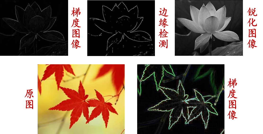
图像锐化：是一种用于改善图像质量的技术，它可以增强图像中的高频细节信息，从而使得图像更加清晰和有视觉冲击力。在图像处理和计算机视觉中，图像锐化通常被用于特征提取、图像增强、目标识别等应用中

一：图像边缘分析

图像边缘分析：是一种用于在图像中找到明显的边缘或轮廓的技术，它可以帮助识别图像中的物体边界、内部结构和纹理等特征。在图像处理和计算机视觉中，边缘分析通常被用于物体检测、目标跟踪、图像分割等应用中

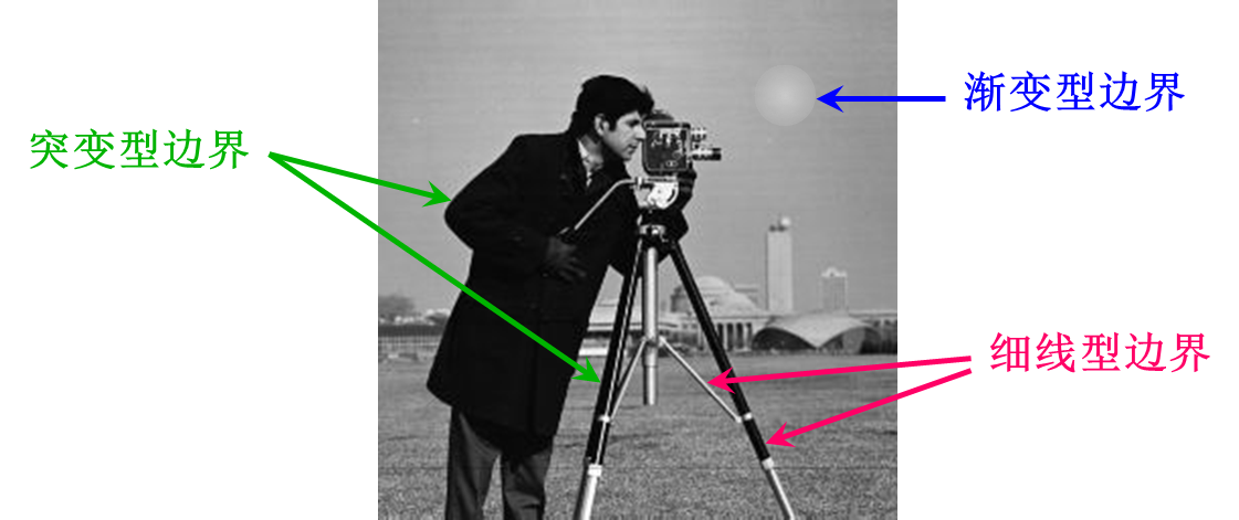
图像中的边缘主要有以下几种类型

• 细线型边缘：
• 突变型边缘：
• 渐变型边缘：

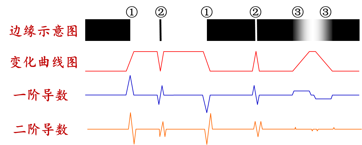
如下图，各种边缘检测方法

• 细线型边缘：检测一阶微分过0点，二阶微分极值点
• 突变型边缘：检测一阶微分极值点，二阶微分过0点
• 渐变型边缘：难检测，二阶微分信息略多于一阶微分

二：一阶微分算子

（1）梯度算子

A：定义

梯度算子：是一类用于图像边缘检测和特征提取的算法，它们基于图像灰度值的变化来计算图像中各个位置的梯度信息，用于找到图像中明显的边缘或特征。对于函数图像$f(x,y)$，它在$(x,y)$处的梯度为

$$G[f(x,y)]={\left[\begin{array}{ll}\frac{\partial f}{\partial x}& \frac{\partial f}{\partial y}\end{array}\right]}^T$$

扫描二维码关注公众号，回复： 15094837 查看本文章

用梯度的幅度来代替，则为

$$G[f(x,y)]={\left[{\left(\frac{\partial f}{\partial x}\right)}^2+{\left(\frac{\partial f}{\partial y}\right)}^2\right]}^{\frac{1}{2}}\text{ 或 }G[f(x,y)]=\left|\frac{\partial f}{\partial x}\right|+\left|\frac{\partial f}{\partial y}\right|$$

离散的数字矩阵，用差分来代替微分，其中$g(x,y)$称为梯度图像

$$\begin{array}{l}\frac{\partial f}{\partial x}=\frac{\Delta f}{\Delta x}=\frac{f(x+1,y)-f(x,y)}{x+1-x}=f(x+1,y)-f(x,y)\\ \frac{\partial f}{\partial y}=\frac{\Delta f}{\Delta y}=\frac{f(x,y+1)-f(x,y)}{y+1-y}=f(x,y+1)-f(x,y)\\ g(x,y)=|f(x+1,y)-f(x,y)|+|f(x,y+1)-f(x,y)|\end{array}$$

B：边缘检测

• 对梯度图像进行阈值化，检测局部变化极值

固定边界灰度：

$$g(x,y)=\{\begin{array}{lc}{L}_G& G[f(x,y)]\ge T\\ f(x,y)& \text{ 其他 }\end{array}$$

突出边界：

$$g(x,y)=\{\begin{array}{lc}G[f(x,y)]& G[f(x,y)]\ge T\\ f(x,y)& \text{ 其他 }\end{array}$$

二值化边界与背景：

$$g(x,y)=\{\begin{array}{lc}{L}_G& G[f(x,y)]\ge T\\ L_B& \text{ 其他 }\end{array}$$

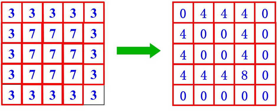
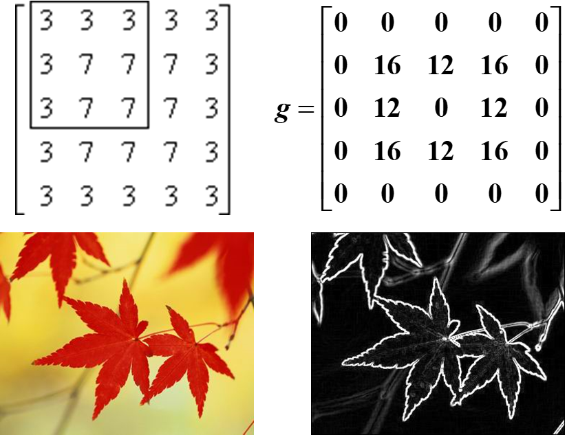
C：示例

如下为一个计算示例

D：程序

---

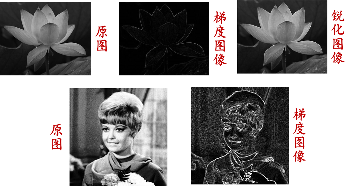
matlab实现：

Image=im2double(rgb2gray(imread('lotus.jpg')));
subplot(131),imshow(Image),title('原图像');
[h,w]=size(Image);
edgeImage=zeros(h,w);
for x=1:w-1
    for y=1:h-1
        edgeImage(y,x)=abs(Image(y,x+1)-Image(y,x))+abs(Image(y+1,x)-Image(y,x));
    end
end
subplot(132),imshow(edgeImage),title('梯度图像');
sharpImage=Image+edgeImage;
subplot(133),imshow(sharpImage),title('锐化图像');

Python实现：

import cv2
import numpy as np
from matplotlib import pyplot as plt

# 读取图像
img = cv2.imread('lotus.jpg')
# 将图像转为灰度图像并将像素值缩放到[0,1]之间
gray = cv2.cvtColor(img, cv2.COLOR_BGR2GRAY)
gray = gray.astype(np.float64) / 255

# 显示原图像
plt.subplot(131)
plt.imshow(gray, cmap='gray')
plt.title('原图像')

# 计算梯度图像
h, w = gray.shape
edge_img = np.zeros((h, w))
for x in range(w-1):
    for y in range(h-1):
        edge_img[y,x] = abs(gray[y,x+1]-gray[y,x]) + abs(gray[y+1,x]-gray[y,x])

# 显示梯度图像
plt.subplot(132)
plt.imshow(edge_img, cmap='gray')
plt.title('梯度图像')

# 锐化图像
sharp_img = gray + edge_img
sharp_img = np.clip(sharp_img, 0, 1)

# 显示锐化图像
plt.subplot(133)
plt.imshow(sharp_img, cmap='gray')
plt.title('锐化图像')

# 显示所有图像
plt.show()

（2）Robert算子

A：定义

Robert算子：是一种边缘检测算子，其原理基于图像中像素值的差异。该算子的实现使用了两个 $2\times 2$ 的卷积核 $G_x$ 和 $G_y$，分别计算像素点 $(x,y)$ 和 $(x+1,y+1)$ 之间的灰度差异。具体来说，$G_x$ 和 $G_y$ 的取值如下

$$\left[\begin{array}{cc}1& 0\\ 0& -1\end{array}\right]和\left[\begin{array}{cc}0& 1\\ -1& 0\end{array}\right]$$

然后，对于输入图像 $I$，可以通过以下公式计算其边缘强度 $E$

• *表示卷积运算

$$E(x,y)=\sqrt{{\left(I(x,y)\ast G_x\right)}^2+{\left(I(x,y)\ast G_y\right)}^2}$$

最终得到的边缘强度 $E$ 可以用来检测图像中的边缘，边缘通常在 $E$ 取得较大值的地方出现。此外，为了提高计算效率，通常也可以使用预先计算好的卷积核来实现 Robert 算子

B：示例

如下图为一计算示例

C：程序

edge函数：用于在图像中检测边缘并生成二值化的边缘图像。该函数语法如下

BW = edge(I, method, threshold, direction)

参数含义如下

• I：输入图像，可以是灰度图像或彩色图像。对于彩色图像，通常会先将其转换为灰度图像，然后再进行边缘检测
• method：边缘检测的方法，包括以下几种，默认值为'sobel'
  • 'sobel'：Sobel算子检测边缘
  • 'prewitt'：Prewitt算子检测边缘
  • 'roberts'：Roberts算子检测边缘
  • 'log'：Laplacian of Gaussian算子检测边缘
  • 'zerocross'：使用Laplacian算子和零交叉检测边缘
  • 'canny'：使用Canny算子检测边缘
• threshold：二值化的阈值，用于将检测到的边缘转换为二值化图像。对于Canny算子，此参数可以是包含两个元素的向量，分别表示低阈值和高阈值。默认值为0.2
• direction：边缘的检测方向，包括以下几种，默认值为'both'
  • 'both'：检测水平和垂直方向的边缘
  • 'horizontal'：仅检测水平方向的边缘
  • 'vertical'：仅检测垂直方向的边缘

---

matlab实现：

Image=im2double(rgb2gray(imread('lotus.jpg')));
% 将名为 lotus.jpg 的彩色图像读入并转换为灰度图像，然后将其类型转换为double型，存储在变量 Image 中。

figure,imshow(Image),title('原图像');
% 显示原始图像

BW= edge(Image,'roberts');
% 对图像进行 Robert 边缘检测，得到一个二值化的边缘图像，存储在变量 BW 中。

figure,imshow(BW),title('边缘检测');
% 显示 Robert 边缘检测结果

H1=[1 0; 0 -1];
H2=[0 1;-1 0];
% 定义两个 2×2 的卷积核 H1 和 H2，分别为 Robert 算子的两个分量。

R1=imfilter(Image,H1);
R2=imfilter(Image,H2);
% 对原始图像分别使用 H1 和 H2 进行卷积操作，得到两个梯度图像 R1 和 R2。

edgeImage=abs(R1)+abs(R2);
% 将 R1 和 R2 两个梯度图像的绝对值相加，得到最终的梯度图像，存储在变量 edgeImage 中。

figure,imshow(edgeImage),title('Robert梯度图像');
% 显示 Robert 算子得到的梯度图像

sharpImage=Image+edgeImage;
% 将原始图像与梯度图像相加，得到锐化后的图像，存储在变量 sharpImage 中。

figure,imshow(sharpImage),title('Robert锐化图像');
% 显示锐化后的图像

Python实现：

import cv2
import numpy as np
from matplotlib import pyplot as plt

# 读入图像并转换为灰度图像
img = cv2.imread('lotus.jpg')
gray = cv2.cvtColor(img, cv2.COLOR_BGR2GRAY)
gray = gray.astype(np.float64) / 255.0

# 显示原图像
plt.imshow(gray, cmap='gray')
plt.title('原图像')
plt.show()

# 进行边缘检测
edge = cv2.Canny(gray, 100, 200)

# 显示边缘检测结果
plt.imshow(edge, cmap='gray')
plt.title('边缘检测')
plt.show()

# 定义两个 2×2 的卷积核 H1 和 H2，分别为 Robert 算子的两个分量
H1 = np.array([[1, 0], [0, -1]])
H2 = np.array([[0, 1], [-1, 0]])

# 对原始图像分别使用 H1 和 H2 进行卷积操作，得到两个梯度图像 R1 和 R2
R1 = cv2.filter2D(gray, -1, H1)
R2 = cv2.filter2D(gray, -1, H2)

# 将 R1 和 R2 两个梯度图像的绝对值相加，得到最终的梯度图像
edgeImage = cv2.addWeighted(cv2.convertScaleAbs(R1), 0.5, cv2.convertScaleAbs(R2), 0.5, 0)

# 显示 Robert 算子得到的梯度图像
plt.imshow(edgeImage, cmap='gray')
plt.title('Robert梯度图像')
plt.show()

# 将原始图像与梯度图像相加，得到锐化后的图像
sharpImage = cv2.addWeighted(gray, 1, edgeImage, 1, 0)

# 显示锐化后的图像
plt.imshow(sharpImage, cmap='gray')
plt.title('Robert锐化图像')
plt.show()

（3）Sobel算子

A：定义

Sobel算子：是一种常用的边缘检测算子，用于在数字图像中检测出边缘部分。它使用两个$3\times 3$的卷积核，分别对图像在$x$和$y$方向进行卷积操作，从而计算出每个像素点处的梯度大小和方向。$x$和$y$方向的卷积核可以表示为

$$H_x=\left[\begin{array}{ccc}-1& -2& -1\\ 0& 0& 0\\ 1& 2& 1\end{array}\right]和H_y=\left[\begin{array}{ccc}-1& 0& 1\\ -2& 0& -2\\ -1& 0& 1\end{array}\right]$$

对于一个灰度图像$I$，对其在$x$方向应用Sobel算子，可以得到一个新的图像$G_x$，其中每个像素的值表示其在$x$方向上的梯度大小，即

$$G_x(i,j)=\sum _{m=-1}^1\sum _{n=-1}^1{H}_x(m+2,n+2)I(i+m,j+n)$$

类似地，对图像$I$在$y$方向应用Sobel算子，可以得到一个新的图像$G_y$，其中每个像素的值表示其在$y$方向上的梯度大小，即

$$G_y(i,j)=\sum _{m=-1}^1\sum _{n=-1}^1{H}_y(m+2,n+2)I(i+m,j+n)$$

最终的梯度图像$G$可以通过$G_x$和$G_y$的平方和再开方得到

$$G(i,j)=\sqrt{G_x(i,j{)}^2+G_y(i,j{)}^2}$$

Sobel算子的目的是找到图像中灰度变化剧烈的位置，也就是边缘。通过比较每个像素点的梯度大小和方向，可以将图像中的边缘部分提取出来，方便后续的图像分析和处理

B：示例

如下图为一计算示例

C：程序

---

matlab实现：

Image=im2double(rgb2gray(imread('lotus.jpg')));
figure,imshow(Image),title('原图像');
BW= edge(Image,'sobel');
figure,imshow(BW),title('边缘检测');
H1=[-1 -2 -1;0 0 0;1 2 1];
H2=[-1 0 1;-2 0 2;-1 0 1];
R1=imfilter(Image,H1);
R2=imfilter(Image,H2);
edgeImage=abs(R1)+abs(R2);
figure,imshow(edgeImage),title('Sobel梯度图像');
sharpImage=Image+edgeImage;
figure,imshow(sharpImage),title('Sobel锐化图像');

Python实现：

import cv2
import numpy as np
import matplotlib.pyplot as plt

# 读入图像并转换为灰度图
image = cv2.imread('lotus.jpg')
image_gray = cv2.cvtColor(image, cv2.COLOR_BGR2GRAY)
image_gray = cv2.normalize(image_gray.astype('float'), None, 0.0, 1.0, cv2.NORM_MINMAX)

# 显示原图像
plt.imshow(image_gray, cmap='gray')
plt.title('原图像')
plt.show()

# 边缘检测
edge_image = cv2.Sobel(image_gray, cv2.CV_64F, 1, 0) + cv2.Sobel(image_gray, cv2.CV_64F, 0, 1)
edge_image = cv2.normalize(np.abs(edge_image), None, 0.0, 1.0, cv2.NORM_MINMAX)

# 显示边缘检测结果
plt.imshow(edge_image, cmap='gray')
plt.title('边缘检测')
plt.show()

# Sobel梯度图像
H1 = np.array([[-1, -2, -1], [0, 0, 0], [1, 2, 1]])
H2 = np.array([[-1, 0, 1], [-2, 0, 2], [-1, 0, 1]])
R1 = cv2.filter2D(image_gray, -1, H1)
R2 = cv2.filter2D(image_gray, -1, H2)
sobel_image = np.abs(R1) + np.abs(R2)
sobel_image = cv2.normalize(sobel_image, None, 0.0, 1.0, cv2.NORM_MINMAX)

# 显示Sobel梯度图像
plt.imshow(sobel_image, cmap='gray')
plt.title('Sobel梯度图像')
plt.show()

# Sobel锐化图像
sharp_image = image_gray + sobel_image
sharp_image = cv2.normalize(sharp_image, None, 0.0, 1.0, cv2.NORM_MINMAX)

# 显示Sobel锐化图像
plt.imshow(sharp_image, cmap='gray')
plt.title('Sobel锐化图像')
plt.show()

（4）Prewitt算子

A：定义

Prewitt算子：是一种经典的图像边缘检测算子，用于检测图像中的水平和垂直边缘。它是一种离散型微分算子，通过对图像像素值的梯度计算来提取边缘信息。对于一个灰度图像 $I$，Prewitt算子分别对图像的水平和垂直方向计算梯度，得到两个梯度图像 $G_x$ 和 $G_y$。这些梯度图像的元素值表示在每个像素处的梯度大小和方向。Prewitt算子的水平和垂直模板分别为

$$H_x=\left[\begin{array}{ccc}-1& 0& 1\\ -1& 0& 1\\ -1& 0& 1\end{array}\right]和H_y=\left[\begin{array}{ccc}-1& -1& -1\\ -0& 0& 0\\ 1& 1& 1\end{array}\right]$$

水平和垂直梯度图像的计算公式为：

• *表示卷积运算

$$G_x=I\ast H_x,G_y=I\ast H_y$$

最后，可以将水平和垂直梯度图像结合起来计算边缘梯度图像 $G$：

$$G=\sqrt{G_x^2+G_y^2}$$

根据梯度大小和方向的信息，可以通过设置一个阈值来判断像素是否为边缘，从而提取出图像中的边缘信息

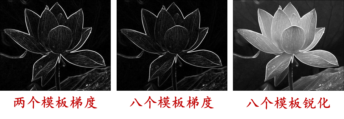
B：示例

C：程序

---

matlab实现：

clear,clc,close all;
Image=im2double(rgb2gray(imread('lotus.jpg')));
H1=[-1 -1 -1;0 0 0;1 1 1];
H2=[0 -1 -1;1 0 -1; 1 1 0];
H3=[1 0 -1;1 0 -1;1 0 -1];
H4=[1 1 0;1 0 -1;0 -1 -1];
H5=[1 1 1;0 0 0;-1 -1 -1];
H6=[0 1 1;-1 0 1;-1 -1 0];
H7=[-1 0 1;-1 0 1;-1 0 1];
H8=[-1 -1 0;-1 0 1;0 1 1];
R1=imfilter(Image,H1);
R2=imfilter(Image,H2);
R3=imfilter(Image,H3);
R4=imfilter(Image,H4);
R5=imfilter(Image,H5);
R6=imfilter(Image,H6);
R7=imfilter(Image,H7);
R8=imfilter(Image,H8);
edgeImage1=abs(R1)+abs(R7);
sharpImage1=edgeImage1+Image;
f1=max(max(R1,R2),max(R3,R4));
f2=max(max(R5,R6),max(R7,R8));
edgeImage2=max(f1,f2);
sharpImage2=edgeImage2+Image;
subplot(221),imshow(edgeImage1),title('两个模板边缘检测');
subplot(222),imshow(edgeImage2),title('八个模板边缘检测');
subplot(223),imshow(sharpImage1),title('两个模板边缘锐化');
subplot(224),imshow(sharpImage2),title('八个模板边缘锐化');

Python实现：

import cv2
import matplotlib.pyplot as plt
import numpy as np

# 读取图像并转换为灰度图像
image = cv2.imread('lotus.jpg')
image = cv2.cvtColor(image, cv2.COLOR_BGR2GRAY)
image = np.float32(image) / 255

# 定义边缘检测和边缘锐化的卷积核
H1 = np.array([[-1, -1, -1], [0, 0, 0], [1, 1, 1]])
H2 = np.array([[0, -1, -1], [1, 0, -1], [1, 1, 0]])
H3 = np.array([[1, 0, -1], [1, 0, -1], [1, 0, -1]])
H4 = np.array([[1, 1, 0], [1, 0, -1], [0, -1, -1]])
H5 = np.array([[1, 1, 1], [0, 0, 0], [-1, -1, -1]])
H6 = np.array([[0, 1, 1], [-1, 0, 1], [-1, -1, 0]])
H7 = np.array([[-1, 0, 1], [-1, 0, 1], [-1, 0, 1]])
H8 = np.array([[-1, -1, 0], [-1, 0, 1], [0, 1, 1]])

# 对图像进行卷积操作，得到八个卷积结果
R1 = cv2.filter2D(image, -1, H1)
R2 = cv2.filter2D(image, -1, H2)
R3 = cv2.filter2D(image, -1, H3)
R4 = cv2.filter2D(image, -1, H4)
R5 = cv2.filter2D(image, -1, H5)
R6 = cv2.filter2D(image, -1, H6)
R7 = cv2.filter2D(image, -1, H7)
R8 = cv2.filter2D(image, -1, H8)

# 计算两个模板和八个模板的边缘检测结果和边缘锐化结果
edgeImage1 = np.abs(R1) + np.abs(R7)
sharpImage1 = edgeImage1 + image
f1 = np.maximum(np.maximum(R1, R2), np.maximum(R3, R4))
f2 = np.maximum(np.maximum(R5, R6), np.maximum(R7, R8))
edgeImage2 = np.maximum(f1, f2)
sharpImage2 = edgeImage2 + image

# 显示图像
plt.subplot(221), plt.imshow(edgeImage1, cmap='gray'), plt.title('两个模板边缘检测')
plt.subplot(222), plt.imshow(edgeImage2, cmap='gray'), plt.title('八个模板边缘检测')
plt.subplot(223), plt.imshow(sharpImage1, cmap='gray'), plt.title('两个模板边缘锐化')
plt.subplot(224), plt.imshow(sharpImage2, cmap='gray',plt.title('八个模板边缘锐化')

三：二阶微分算子

（1）定义

二阶微分算子（拉普拉斯算子）：在三维欧几里得空间中，拉普拉斯算子通常表示为 $\Delta$，它可以被定义为向量算子 $\nabla$ 的散度的运算，即

$${\Delta }^{2}f=\frac{{\partial }^{2}f}{\partial x^2}+\frac{{\partial }^{2}f}{\partial y^2}$$

其中

$$\begin{array}{rl}\frac{{\partial }^{2}f}{\partial x^2}& ={\Delta }_{x}f(x+1,y)-{\Delta }_{x}f(x,y)\\ & =[f(x+1,y)-f(x,y)]-[f(x,y)-f(x-1,y)]\\ & =f(x+1,y)+f(x-1,y)-2f(x,y)\\ \frac{{\partial }^{2}f}{\partial y^2}& ={\Delta }_{y}f(x,y+1)-{\Delta }_{y}f(x,y)\\ & =[f(x,y+1)-f(x,y)]-[f(x,y)-f(x,y-1)]\\ & =f(x,y+1)+f(x,y-1)-2f(x,y)\end{array}$$

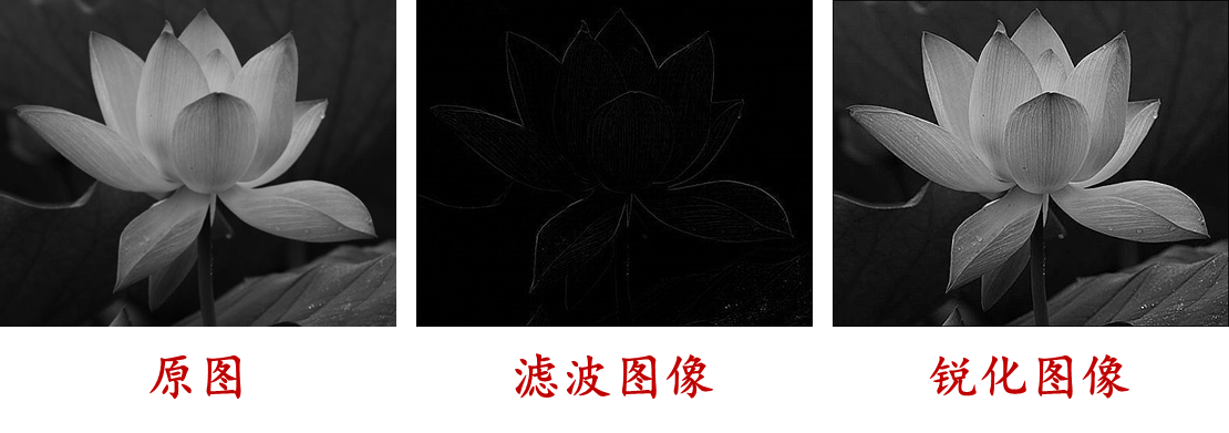
（2）示例

如下图为示例

（3）程序

---

matlab实现：

Image=im2double(rgb2gray(imread('lotus.jpg')));
figure,imshow(Image),title('原图像');
H=fspecial('laplacian',0);
R=imfilter(Image,H);
edgeImage=abs(R);
figure,imshow(edgeImage),title('Laplacian梯度图像');
H1=[0 -1 0;-1 5 -1;0 -1 0];
sharpImage=imfilter(Image,H1);
figure,imshow(sharpImage),title('Laplacian锐化图像');

Python实现：

import cv2
import matplotlib.pyplot as plt

Image = cv2.imread('lotus.jpg')
Image = cv2.cvtColor(Image, cv2.COLOR_BGR2GRAY)
Image = cv2.normalize(Image.astype('float'), None, 0.0, 1.0, cv2.NORM_MINMAX)

plt.imshow(Image, cmap='gray')
plt.title('原图像')
plt.show()

H = cv2.Laplacian(Image, ddepth=-1, ksize=3)
R = cv2.filter2D(Image, -1, H)

edgeImage = cv2.convertScaleAbs(R)

plt.imshow(edgeImage, cmap='gray')
plt.title('Laplacian梯度图像')
plt.show()

H1 = np.array([[0, -1, 0], [-1, 5, -1], [0, -1, 0]])
sharpImage = cv2.filter2D(Image, -1, H1)

plt.imshow(sharpImage, cmap='gray')
plt.title('Laplacian锐化图像')
plt.show()