在这篇博文中,将针对具有 80 个标签的 coco 数据集逐行解释 Yolov3 预训练对象检测的代码说明。
我们可以从 yolo 官网获取 weights 文件和 cfg 文件:https://pjreddie.com/darknet/yolo/
image = cv2.imread('./testing images/crosswalk-featured.jpg')
#cv2.imshow('image',image)
#cv2.waitKey()
#cv2.destroyAllWindows()
original_with , original_height = image.shape[1] , image.shape[0]

Neural_Network = cv2.dnn.readNetFromDarknet('./Files/yolov3.cfg','./Files/yolov3.weights')
classes_names = []
k = open('./Files/class_names','r')
for i in k.readlines():
    classes_names.append(i.strip())
#print(classes_names)
blob = cv2.dnn.blobFromImage(image , 1/255 , (320,320) , True , crop = False)
#print(blob.shape)
Neural_Network.setInput(blob)
cfg_data = Neural_Network.getLayerNames()
#print(cfg_data)
layer_names = Neural_Network.getUnconnectedOutLayers()
outputs = [cfg_data[i-1] for i in layer_names]
#print(outputs)
output_data = Neural_Network.forward(outputs)
prediction_box , bounding_box , confidence , class_labels = bounding_box_prediction(output_data)
final_prediction(prediction_box , bounding_box , confidence , class_labels , original_with / 320 , original_height / 320 )
第一行从
testing images目录中读取图像文件crosswalk-featured.jpg并将其作为数组存储在变量image中。接下来的两行注释:使用 OpenCV 显示图像
下一行检索图像的尺寸(宽度和高度)并将它们分别存储在
original_with和original_height变量中。cv2.dnn.readNetFromDarknet('./Files/yolov3.cfg','./Files/yolov3.weights'):从 Darknet 框架加载预训练的 YOLOv3 模型。这两个参数分别是配置文件和权重文件的路径。接下来的几行从文件中读取 COCO 数据集的类名
class_names,并将它们存储在列表classes_names中。cv2.dnn.blobFromImage()函数根据输入图像创建一个 4 维blob。blob 是神经网络期望作为输入的标准化格式。传递的参数是输入图像、比例因子、输出大小和平均相减值。神经网络的函数
setInput()用于将输入 blob 设置为网络的输入。getLayerNames()函数返回神经网络中所有层的名称。getUnconnectedOutLayers()函数返回未连接到任何其他层的输出层的索引。在 YOLOv3 模型中,输出层索引为 82、94 和 106。forward()函数用于执行神经网络的前向传递,并获得给定输入 blob 的输出预测。outputs 变量是未连接输出层的输出列表。调用
bounding_box_prediction()函数,它使用 IOU(并集交集)技术从输出预测中提取边界框坐标、类标签和置信度分数。调用
final_prediction()函数以在输入图像上绘制预测的边界框,以及预测的类标签和置信度分数。original_with / 320和original_height / 320是用于将边界框坐标转换为输入图像原始大小的缩放因子。
def bounding_box_prediction(output_data):
    bounding_box = []
    class_labels = []
    confidence_score = []
    for i in output_data:
        for j in i:
            high_label = j[5:]
            classes_ids = np.argmax(high_label)
            confidence = high_label[classes_ids]

            if confidence > Threshold:
                w , h = int(j[2] * image_size) , int(j[3] * image_size)
                x , y = int(j[0] * image_size - w/2) , int(j[1] * image_size - h/2)
                bounding_box.append([x,y,w,h])
                class_labels.append(classes_ids)
                confidence_score.append(confidence)

    prediction_boxes = cv2.dnn.NMSBoxes(bounding_box , confidence_score , Threshold , .6)
return prediction_boxes , bounding_box ,confidence_score,class_labels函数bounding_box_prediction()用于获取每个检测到的对象的边界框、类标签和置信度分数。
它接受output_data(YOLOv3 神经网络的输出)作为参数。
在函数内部,将迭代每个元素output_data以获取边界框坐标、类标签和置信度分数。
使用argmax()以获得最高置信度分数的索引。如果置信度分数高于Threshold,则边界框坐标、类标签和置信度分数将附加到它们各自的列表中。
最后,使用cv2.dnn.NMSBoxes 将非最大抑制算法应用于边界框。
import numpy as np
import pandas as pd
import matplotlib.pyplot as plt


font = cv2.FONT_HERSHEY_COMPLEX

Threshold = 0.5
image_size = 320


def final_prediction(prediction_box , bounding_box , confidence , class_labels,width_ratio,height_ratio):
    for j in prediction_box.flatten():
        x, y , w , h = bounding_box[j]
        x = int(x * width_ratio)
        y = int(y * height_ratio)
        w = int(w * width_ratio)
        h = int(h * height_ratio)

        label = str(classes_names[class_labels[j]])
        conf_ = str(round(confidence[j],2))
        cv2.rectangle(image , (x,y) , (x+w , y+h) , (0,0,255) , 2)
        cv2.putText(image , label+' '+conf_ , (x , y-2) , font , .2 , (0,255,0),1)
在本部分中,我们将为模型导入一些必要的库,包括 NumPy、Pandas 和 Matplotlib,并设置用于显示检测到的对象的标签和置信度分数的字体。
Threshold变量设置置信度分数的最小阈值,而image_size变量是要处理的图像的大小。
函数final_prediction()用于在检测到的对象周围绘制边界框并显示标签和置信度分数。它接受的参数为:
prediction_box:NMS 算法的输出bounding_box:边界框的坐标confidence:检测到的对象的置信度分数class_labels:检测到的对象的类标签width_ratio:原始图像宽度与处理后图像的比率height_ratio:原始图像高度与处理后图像高度的比率
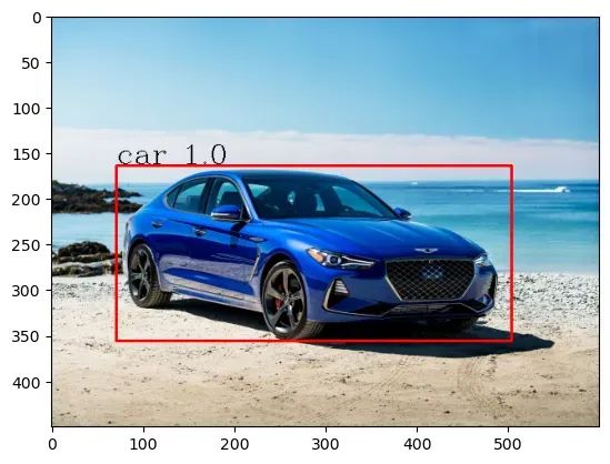
测试图像:

完整代码:
import numpy as np
import pandas as pd
import matplotlib.pyplot as plt


font = cv2.FONT_HERSHEY_COMPLEX

Threshold = 0.5
image_size = 320


def final_prediction(prediction_box , bounding_box , confidence , class_labels,width_ratio,height_ratio):
    for j in prediction_box.flatten():
        x, y , w , h = bounding_box[j]
        x = int(x * width_ratio)
        y = int(y * height_ratio)
        w = int(w * width_ratio)
        h = int(h * height_ratio)

        label = str(classes_names[class_labels[j]])
        conf_ = str(round(confidence[j],2))
        cv2.rectangle(image , (x,y) , (x+w , y+h) , (0,0,255) , 2)
        cv2.putText(image , label+' '+conf_ , (x , y-2) , font , .2 , (0,255,0),1)

def bounding_box_prediction(output_data):
    bounding_box = []
    class_labels = []
    confidence_score = []
    for i in output_data:
        for j in i:
            high_label = j[5:]
            classes_ids = np.argmax(high_label)
            confidence = high_label[classes_ids]

            if confidence > Threshold:
                w , h = int(j[2] * image_size) , int(j[3] * image_size)
                x , y = int(j[0] * image_size - w/2) , int(j[1] * image_size - h/2)
                bounding_box.append([x,y,w,h])
                class_labels.append(classes_ids)
                confidence_score.append(confidence)

    prediction_boxes = cv2.dnn.NMSBoxes(bounding_box , confidence_score , Threshold , .6)
    return prediction_boxes , bounding_box ,confidence_score,class_labels


image = cv2.imread('./testing images/crosswalk-featured.jpg')
#cv2.imshow('image',image)
#cv2.waitKey()
#cv2.destroyAllWindows()
original_with , original_height = image.shape[1] , image.shape[0]

Neural_Network = cv2.dnn.readNetFromDarknet('./Files/yolov3.cfg','./Files/yolov3.weights')
classes_names = []
k = open('./Files/class_names','r')
for i in k.readlines():
    classes_names.append(i.strip())
#print(classes_names)
blob = cv2.dnn.blobFromImage(image , 1/255 , (320,320) , True , crop = False)
#print(blob.shape)
Neural_Network.setInput(blob)
cfg_data = Neural_Network.getLayerNames()
#print(cfg_data)
layer_names = Neural_Network.getUnconnectedOutLayers()
outputs = [cfg_data[i-1] for i in layer_names]
#print(outputs)
output_data = Neural_Network.forward(outputs)
prediction_box , bounding_box , confidence , class_labels = bounding_box_prediction(output_data)
final_prediction(prediction_box , bounding_box , confidence , class_labels , original_with / 320 , original_height / 320 )
Yolov3检测:
你可以从这里获得完整的 Yolov3 架构解释:
https://medium.com/p/74cf9ade2044/edit
☆ END ☆
如果看到这里,说明你喜欢这篇文章,请转发、点赞。微信搜索「uncle_pn」,欢迎添加小编微信「 woshicver」,每日朋友圈更新一篇高质量博文。
↓扫描二维码添加小编↓
