文章目录
前言
记录在tf1.x与tf2.x中使用卷积神经网络完成CIFAR-10数据集识别多分类任务,并进行断点续训。
一、卷积神经网络CNN
1、全连接网络:参数增多,速度减慢,过拟合
2、卷积神经网络:每层由多个二维平面组成,每个平面由多个独立神经元组成
输入层→(卷积层+→池化层?)+→全连接层+
(1)卷积层:增强特征,降低噪音
#卷积
y = tf.nn.conv2d(x, w, strides, padding) + b
'''
x:输入4维张量[batch,height,weight,channel]
w:[height,weight,input_channel,output_channel]
b:output_channel
strides:每一维步长
'''
#卷积层
tf.keras.layers.Conv2D(filters,#卷积核数目
					   kernel_size,#卷积核大小
          			   activation,#激活函数
          			   padding#填充方式))
图像 ⟶ 卷积核 权值矩阵 特征图 图像\underset{权值矩阵}{\overset{卷积核}{\longrightarrow}}特征图 图像权值矩阵⟶卷积核特征图
局部连接,权值共享
步长:卷积核移动格数,得到不同尺寸输出(降采样)
[ N 1 , N 1 ] ⟶ [ N 1 , N 1 ] S [ ( N 1 − N 2 ) / S + 1 , ( N 1 − N 2 ) / S + 1 ] [N1,N1]\underset{S}{\overset{[N1,N1]}{\longrightarrow}}[(N1-N2)/S+1,(N1-N2)/S+1] [N1,N1]S⟶[N1,N1][(N1−N2)/S+1,(N1−N2)/S+1]
0填充:用0填充边缘,使输入输出大小相同
多通道卷积:使用多个卷积核提取特征
(2)降采样层:减少参数,降低过拟合
#池化
y1 = tf.nn.max_pool(y, ksize, strides, padding)
'''
y:输入4维张量[batch,height,weight,channel]
ksize:池化窗口[1,height,weight,1]
'''
#池化层
tf.keras.layers.MaxPooling2D(pool_size)
池化:计算区域均值(背景特征)或最大值(纹理特征),合并特征
二、Tensorflow1.x
1.加载数据集
在tensorflow2.x中调用CIFAR-10数据集
10分类32x32RGB彩色图片,训练集50000张,测试集10000张
x_train:(50000, 32, 32, 3)
y_train:(10000, 1)
x_test:(10000, 32, 32, 3)
y_test:(10000, 1)
import tensorflow as tf2
import matplotlib.pyplot as plt
import numpy as np
cifar10 = tf2.keras.datasets.cifar10
(x_train, y_train), (x_test, y_test) = cifar10.load_data()
#显示16张图片
def show(images, labels, preds):
    label_dict = {

    0:'plane', 1:'car', 2:'bird', 3:'cat',\
                  4:'deer', 5:'dog', 6:'frog', 7:'horse',\
                  8:'ship', 9:'trunk'}
    fig1 = plt.figure(1, figsize=(12, 12))
    for i in range(16):
        ax = fig1.add_subplot(4, 4, i+1)
        ax.imshow(images[i], cmap='binary')
        label = label_dict[np.argmax(labels[i])]
        pred = label_dict[np.argmax(preds[i])]
        title = 'label:%s,pred:%s' % (label, pred)
        ax.set_title(title)
        ax.set_xticks([])
        ax.set_yticks([])
2.数据处理
import tensorflow.compat.v1 as tf
from sklearn.preprocessing import OneHotEncoder
from sklearn.utils import shuffle
from time import time
import os
tf.disable_eager_execution()

#维度转换,灰度值归一化,标签独热编码
x_train = (x_train/255.0).astype(np.float32)
x_test = (x_test/255.0).astype(np.float32)
y_train = OneHotEncoder().fit_transform(y_train).toarray()
y_test = OneHotEncoder().fit_transform(y_test).toarray()
#训练集50000个样本,取5000个样本作为验证集;测试集10000个样本
x_valid, y_valid = x_train[45000:], y_train[45000:]
x_train, y_train = x_train[:45000], y_train[:45000]
3.定义模型
#输入层
#输入通道3,图像大小32*32
with tf.name_scope('Input'):
    x = tf.placeholder(tf.float32, [None, 32, 32, 3], name='X')
#卷积层1
#输出通道32,卷积核3*3,步长为1,图像大小32*32
with tf.name_scope('Conv_1'):
    w1 = tf.Variable(\
         tf.truncated_normal((3,3,3,32), stddev=0.1), name='W1')
    b1 = tf.Variable(tf.zeros(32), name='B1')
    y1 = tf.nn.conv2d(x, w1, strides=[1,1,1,1], padding='SAME') + b1
    y1 = tf.nn.relu(y1)
#池化层1
#输出通道32,最大值池化2*2,步长为2,图像大小16*16
with tf.name_scope('Pool_1'):
    y2 = tf.nn.max_pool(y1, ksize=[1,2,2,1], strides=[1,2,2,1], padding='SAME')
#卷积层2
#输出通道64,卷积核3*3,步长为1,图像大小32*32
with tf.name_scope('Conv_1'):
    w3 = tf.Variable(\
         tf.truncated_normal((3,3,32,64), stddev=0.1), name='W3')
    b3 = tf.Variable(tf.zeros(64), name='B3')
    y3 = tf.nn.conv2d(y2, w3, strides=[1,1,1,1], padding='SAME') + b3
    y3 = tf.nn.relu(y3)
#池化层2
#输出通道64,最大值池化2*2,步长为2,图像大小8*8
with tf.name_scope('Pool_1'):
    y4 = tf.nn.max_pool(y3, ksize=[1,2,2,1], strides=[1,2,2,1], padding='SAME')
#全连接层
#输入8*8*64,128个神经元
with tf.name_scope('Output'):
    w5 = tf.Variable(\
         tf.truncated_normal((8*8*64, 128), stddev=0.1), name='W5')
    b5 = tf.Variable(tf.zeros((128)), name='B5')
    y5 = tf.reshape(y4, (-1, 8*8*64))
    y5 = tf.matmul(y5, w5) + b5
    y5 = tf.nn.relu(y5)
    y5 = tf.nn.dropout(y5, keep_prob=0.8)
#输出层
#输出10个神经元
with tf.name_scope('Output'):
    w6 = tf.Variable(\
         tf.truncated_normal((128, 10), stddev=0.1), name='W6')
    b6 = tf.Variable(tf.zeros((10)), name='B6')
    pred = tf.matmul(y5, w6) + b6
    #pred = tf.nn.softmax(y6)
#优化器
with tf.name_scope('Optimizer'):
    y = tf.placeholder(tf.float32, [None, 10], name='Y')
    loss_function = tf.reduce_mean(\
                    tf.nn.softmax_cross_entropy_with_logits(\
                    logits=pred, labels=y))
    optimizer = tf.train.AdamOptimizer(learning_rate=0.001)\
                .minimize(loss_function)
#准确率
equal = tf.equal(tf.argmax(y, axis=1), tf.argmax(pred, axis=1))
accuracy = tf.reduce_mean(tf.cast(equal, tf.float32))
4.训练模型
训练参数
train_epoch = 10
batch_size = 1000
batch_num = x_train.shape[0] // batch_size
#损失函数与准确率
step = 0
display_step = 10
loss_list = []
acc_list = []
epoch = tf.Variable(0, name='epoch', trainable=False)
#变量初始化
sess = tf.Session()
init = tf.global_variables_initializer()
sess.run(init)
断点续训
ckpt_dir = './ckpt_dir/cifar10'
if not os.path.exists(ckpt_dir):
    os.makedirs(ckpt_dir)
vl = [v for v in tf.global_variables() if 'Adam' not in v.name]
saver = tf.train.Saver(var_list=vl, max_to_keep=1)
ckpt = tf.train.latest_checkpoint(ckpt_dir)
if ckpt != None:
    saver.restore(sess, ckpt)
start_ep = sess.run(epoch)
迭代训练
start_time = time()
for ep in range(start_ep, train_epoch):
    #打乱顺序
    x_train, y_train = shuffle(x_train, y_train)
    print('epoch:{}/{}'.format(ep+1, train_epoch))
    for batch in range(batch_num):
        xi = x_train[batch*batch_size:(batch+1)*batch_size]
        yi = y_train[batch*batch_size:(batch+1)*batch_size]
        sess.run(optimizer, feed_dict={

    x:xi, y:yi})
        step = step + 1
        if step % display_step == 0:
            loss, acc = sess.run([loss_function, accuracy],\
                                 feed_dict={

    x:x_valid, y:y_valid})
            loss_list.append(loss)
            acc_list.append(acc)
    #保存检查点
    sess.run(epoch.assign(ep+1))
    saver.save(sess, os.path.join(ckpt_dir,\
              'cifar10_model.ckpt'), global_step=ep+1)
5.结果可视化
end_time = time()
y_pred, acc = sess.run([pred, accuracy],\
                        feed_dict={

    x:x_test, y:y_test})
fig2 = plt.figure(2, figsize=(12, 6))
ax = fig2.add_subplot(1, 2, 1)
ax.plot(loss_list, 'r-')
ax.set_title('loss')
ax = fig2.add_subplot(1, 2, 2)
ax.plot(acc_list, 'b-')
ax.set_title('acc')
print('用时%.1fs' % (end_time - start_time))
print('Accuracy:{:.2%}'.format(acc))
show(x_test[0:16], y_test[0:16], y_pred[0:16])
在第8次训练后中断,再次运行,从第9次开始训练

验证集上的损失与准确率

前16张图片的标签与预测值

二、Tensorflow2.x
1.加载数据集
标签值采用整数,不进行独热编码
import tensorflow as tf
import matplotlib.pyplot as plt
import numpy as np
from time import time
cifar10 = tf.keras.datasets.cifar10
(x_train, y_train), (x_test, y_test) = cifar10.load_data()
#显示16张图片
def show(images, labels, preds):
    label_dict = {

    0:'plane', 1:'car', 2:'bird', 3:'cat',\
                  4:'deer', 5:'dog', 6:'frog', 7:'horse',\
                  8:'ship', 9:'trunk'}
    fig1 = plt.figure(1, figsize=(12, 12))
    for i in range(16):
        ax = fig1.add_subplot(4, 4, i+1)
        ax.imshow(images[i], cmap='binary')
        label = label_dict[labels[i]]
        pred = label_dict[preds[i]]
        title = 'label:%s,pred:%s' % (label, pred)
        ax.set_title(title)
        ax.set_xticks([])
        ax.set_yticks([])
2.数据处理
不进行验证集的划分
#维度转换,灰度值归一化,标签独热编码
x_train = (x_train/255.0).astype(np.float32)
x_test = (x_test/255.0).astype(np.float32)
3.定义模型
创建模型
model = tf.keras.models.Sequential()
#添加层
model.add(tf.keras.layers.Conv2D(filters=32, kernel_size=(3,3),\
          input_shape=(32,32,3), activation='relu', padding='same'))
model.add(tf.keras.layers.Dropout(rate=0.3))
model.add(tf.keras.layers.MaxPooling2D(pool_size=(2,2)))
model.add(tf.keras.layers.Conv2D(filters=64, kernel_size=(3,3),\
          activation='relu', padding='same'))
model.add(tf.keras.layers.Dropout(rate=0.3))
model.add(tf.keras.layers.MaxPooling2D(pool_size=(2,2)))
model.add(tf.keras.layers.Flatten())
model.add(tf.keras.layers.Dense(units=10,\
          kernel_initializer='normal', activation='softmax'))
#模型摘要
model.summary()
加载模型
'''
#加载模型(整个模型)
mpath = './model/cifar10.h5'
model.load_weights(mpath)
'''
#加载模型(检查点)
cdir = './model/'
ckpt = tf.train.latest_checkpoint(cdir)
if ckpt != None:
    model.load_weights(ckpt)
训练模式
#整数类型作标签
model.compile(optimizer='adam',\
              loss='sparse_categorical_crossentropy',\
              metrics=['accuracy'])
4.训练模型
#回调参数设置检查点与早停
cpath = './model/cifar10.{epoch:02d}-{val_loss:.4f}.H5'
callbacks = [tf.keras.callbacks.ModelCheckpoint(filepath=cpath,
                                                save_weights_only=True,
                                                verbose=1,
                                                save_freq='epoch'),
             tf.keras.callbacks.EarlyStopping(monitor='val_loss',
                                              patience=3)]
#模型训练
start_time = time()
history = model.fit(x_train, y_train,\
                    validation_split=0.2, epochs=10, batch_size=1000,\
                    callbacks=callbacks, verbose=1)
end_time = time()
print('用时%.1fs' % (end_time-start_time))
5.结果可视化
history.history:字典类型数据
loss,accuracy,val_loss,val_accuracy
fig2 = plt.figure(2, figsize=(12, 6))
ax = fig2.add_subplot(1, 2, 1)
ax.plot(history.history['val_loss'], 'r-')
ax.set_title('loss')
ax = fig2.add_subplot(1, 2, 2)
ax.plot(history.history['val_accuracy'], 'b-')
ax.set_title('acc')
模型评估
test_loss, test_acc = model.evaluate(x_train, y_train, verbose=1)
print('Loss:%.2f' % test_loss)
print('Accuracy:{:.2%}'.format(test_acc))
模型预测
#分类预测
preds = model.predict_classes(x_test)
show(x_test[0:16], y_test[0:16].flatten(), preds[0:16])
#保存模型
#model.save_weights(mpath)
网络结构

训练后保存模型

验证集损失值与准确率

前16张图片的标签值与预测值

导入模型,准确率与之前相同

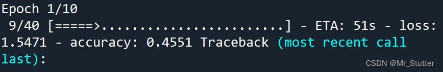
在第二批训练后停止程序

再次训练时准确率在之前的基础上提升
总结
卷积神经网络能够对数据进行特征提取,减少参数的数量,提高训练速度;
使用OneHotEncoder进行独热编码后需要使用toarray()转化为数组形式参与运算;
在训练时间较长时可定时保存进行断点续训;
在tf1.x中保存检查点时会保存多个同名的权重,可不保存名称中含有Adam的权重,保存前后需要重启控制台以避免加载时权重名称不对应。