一、选题的背景
橄榄球起源于足球,二者即相似又有所区别。计算机技术发展至今,AI技术也有了极大的进步,通过机器学习不断的训练,AI对于足球和橄榄球的识别能力可以帮助人们对足球和橄榄球的分辨。机器学习是一种智能技术,对足球和橄榄球的分类识别,可以帮助我们了解足球和橄榄球的差异特征,使用机器学习技术来分析这些差异特征,从而提高计算机对足球和橄榄球的识别能力。
二、机器学习案例设计方案
从网站中下载相关的数据集,对数据集进行整理,给数据集中的文件打上标签,在python的环境中,对数据进行预处理,利用keras,构建网络,训练模型,将训练过程产生的数据保存为h5文件,查看验证集的损失和准确率,绘制训练过程中的损失曲线和精度曲线,从测试集中读取一条样本,建立模型,输入为原图像,输出为原模型的前8层的激活输出的特征图,显示第一层激活输出特的第一个滤波器的特征图,读取图像样本,改变其尺寸,导入图片测试模型。
数据集介绍:图像中可能有不同的方面帮助将其识别为足球和橄榄球,可能是球的形状或球员的服装。由于正在研究图像分类问题,我将数据结构分为:训练文件夹有2448张图片,足球和橄榄球两个类别都有1224张图片,验证文件夹有610张图片,足球和橄榄球两个类别都有350张图片,测试文件夹有20张图片。
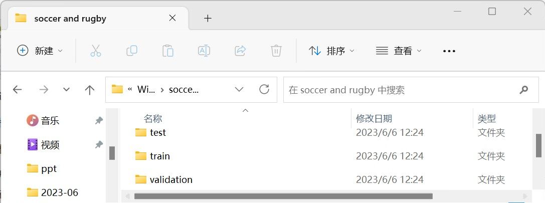
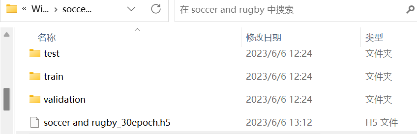
数据结构如下:
输入–3078
-----训练–2448
------------足球–1224
------------橄榄球–1224
-----验证–610
------------足球–305
------------橄榄球–305
-----测试–20
数据集来源:极市平台https://www.cvmart.net/dataSets
三、机器学习的实现步骤
1.下载数据集
2.检查一下,看看每个分组(训练 / 验证 / 测试)中分别包含多少张图像

#检查一下,看看每个分组(训练 / 验证 / 测试)中分别包含多少张图像
import os
train_path="C:/soccer and rugby/train/"
print('足球的训练集图像数量:', len(os.listdir(train_path+"soccer")))
print('橄榄球的训练集图像数量:', len(os.listdir(train_path+"rugby")))
print('-----------------------------------')
valid_path="C:/soccer and rugby/validation/"
print('足球的验证集图像数量:', len(os.listdir(valid_path+"soccer")))
print('橄榄球的验证集图像数量:', len(os.listdir(valid_path+"rugby")))
print('-----------------------------------')
test_path="C:/soccer and rugby/test/"
print('测试集图像数量:', len(os.listdir(test_path)))


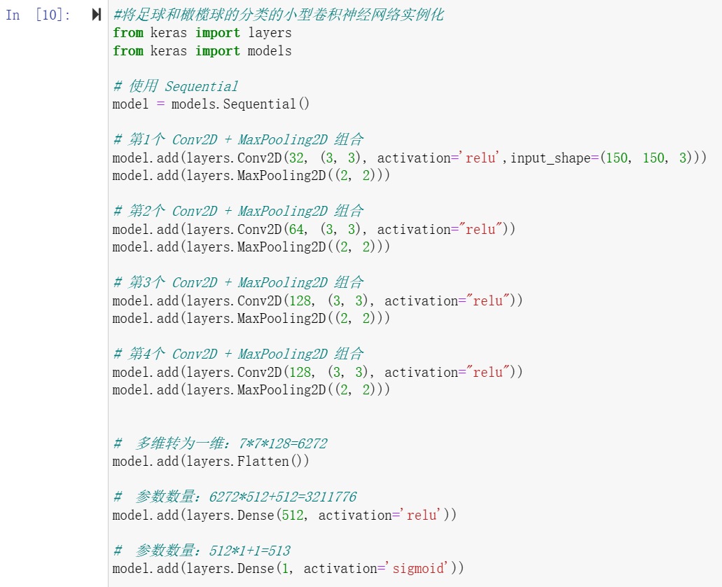
3.将足球和橄榄球的分类的小型卷积神经网络实例化

#将足球和橄榄球的分类的小型卷积神经网络实例化
from keras import layers
from keras import models

# 使用 Sequential
model = models.Sequential()

# 第1个 Conv2D + MaxPooling2D 组合
model.add(layers.Conv2D(32, (3, 3), activation='relu',input_shape=(150, 150, 3)))
model.add(layers.MaxPooling2D((2, 2)))

# 第2个 Conv2D + MaxPooling2D 组合
model.add(layers.Conv2D(64, (3, 3), activation="relu"))
model.add(layers.MaxPooling2D((2, 2)))

# 第3个 Conv2D + MaxPooling2D 组合
model.add(layers.Conv2D(128, (3, 3), activation="relu"))
model.add(layers.MaxPooling2D((2, 2)))

# 第4个 Conv2D + MaxPooling2D 组合
model.add(layers.Conv2D(128, (3, 3), activation="relu"))
model.add(layers.MaxPooling2D((2, 2)))


#  多维转为一维:7*7*128=6272
model.add(layers.Flatten())

#  参数数量:6272*512+512=3211776
model.add(layers.Dense(512, activation='relu'))

#  参数数量:512*1+1=513
model.add(layers.Dense(1, activation='sigmoid'))

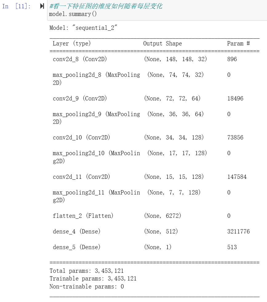
4.看一下特征图的维度如何随着每层变化
#看一下特征图的维度如何随着每层变化
model.summary()
5.编译模型

# 编译模型
# RMSprop 优化器。因为网络最后一层是单一sigmoid单元,
# 所以使用二元交叉熵作为损失函数
from keras import optimizers

model.compile(loss='binary_crossentropy',
              optimizer=optimizers.RMSprop(lr=1e-4),
              metrics=['acc'])


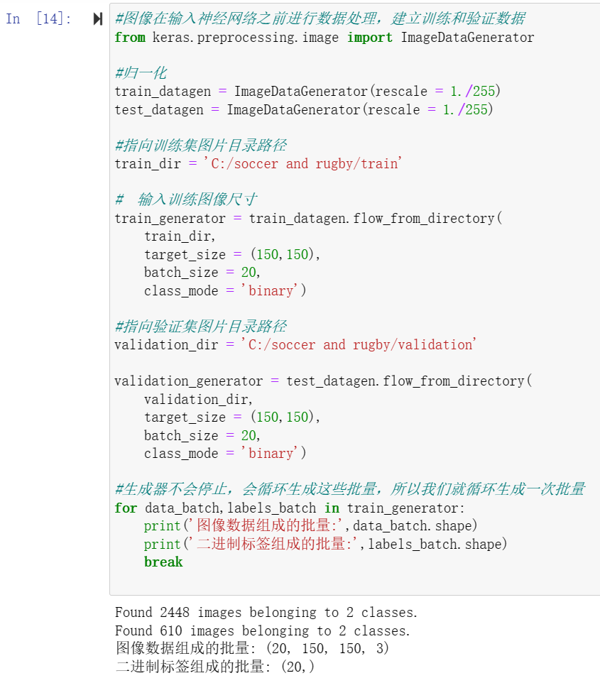
6.图像在输入神经网络之前进行数据处理,建立训练和验证数据

#图像在输入神经网络之前进行数据处理,建立训练和验证数据
from keras.preprocessing.image import ImageDataGenerator

#归一化
train_datagen = ImageDataGenerator(rescale = 1./255)
test_datagen = ImageDataGenerator(rescale = 1./255)

#指向训练集图片目录路径
train_dir = 'C:/soccer and rugby/train'

#  输入训练图像尺寸
train_generator = train_datagen.flow_from_directory(
    train_dir,
    target_size = (150,150),
    batch_size = 20,
    class_mode = 'binary')

#指向验证集图片目录路径
validation_dir = 'C:/soccer and rugby/validation'

validation_generator = test_datagen.flow_from_directory(
    validation_dir,
    target_size = (150,150),
    batch_size = 20,
    class_mode = 'binary')

#生成器不会停止,会循环生成这些批量,所以我们就循环生成一次批量
for data_batch,labels_batch in train_generator:
    print('图像数据组成的批量:',data_batch.shape)
    print('二进制标签组成的批量:',labels_batch.shape)
    break

7.训练模型30轮次

#训练模型30轮次
history = model.fit(
                    train_generator,
                    steps_per_epoch = 100,
#训练30次
                    epochs = 30,
                    validation_data = validation_generator,
                    validation_steps = 50

8.将训练过程产生的数据保存为h5文件

#将训练过程产生的数据保存为h5文件
from keras.models import load_model
model.save('C:/soccer and rugby/soccer and rugby_30epoch.h5')

#如何打开.h5文件
from keras.models import load_model
from keras import layers
from keras import models

model=load_model('C:/soccer and rugby/soccer and rugby_30epoch.h5')


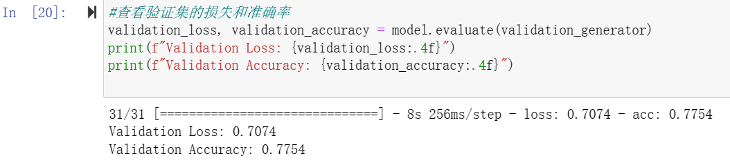
9.查看验证集的损失和准确率
#查看验证集的损失和准确率
validation_loss, validation_accuracy = model.evaluate(validation_generator)
print(f"Validation Loss: {validation_loss:.4f}")
print(f"Validation Accuracy: {validation_accuracy:.4f}")
10.绘制训练过程中的损失曲线和精度曲线

#绘制训练过程中的损失曲线和精度曲线
import matplotlib.pyplot as plt

acc = history.history['acc']
loss =history.history['loss']

epochs = range(1,len(acc) + 1)

plt.plot(epochs,acc,'bo',label='Training acc')
plt.plot(epochs,loss,'b',label='loss')
plt.title('Training and validation accuracy')
plt.legend()
#绘制训练过程中的损失曲线
import matplotlib.pyplot as plt

loss =history.history['loss']
epochs = range(1,len(acc) + 1)
plt.plot(epochs,loss,'b',label='loss')
plt.title('loss')
plt.legend()
#绘制训练过程中精度曲线
import matplotlib.pyplot as plt
acc = history.history['acc']
epochs = range(1,len(acc) + 1)

plt.plot(epochs,acc,'bo',label='Training acc')
plt.title(' accuracy')
plt.legend()


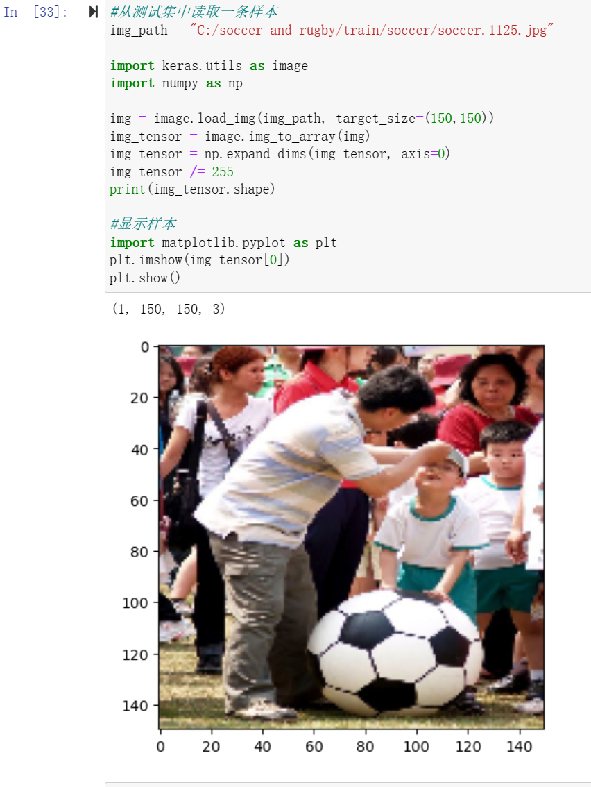
11.从测试集中读取一条样本并显示

#从测试集中读取一条样本
img_path = "C:/soccer and rugby/train/soccer/soccer.1125.jpg"

import keras.utils as image
import numpy as np

img = image.load_img(img_path, target_size=(150,150))
img_tensor = image.img_to_array(img)
img_tensor = np.expand_dims(img_tensor, axis=0)
img_tensor /= 255
print(img_tensor.shape)

#显示样本
import matplotlib.pyplot as plt
plt.imshow(img_tensor[0])
plt.show()

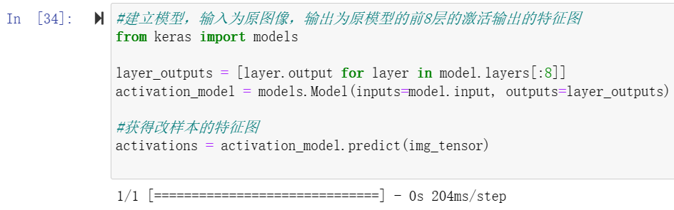
12.建立模型,输入为原图像,输出为原模型的前8层的激活输出的特征图

#建立模型,输入为原图像,输出为原模型的前8层的激活输出的特征图
from keras import models

layer_outputs = [layer.output for layer in model.layers[:8]]
activation_model = models.Model(inputs=model.input, outputs=layer_outputs)

#获得改样本的特征图
activations = activation_model.predict(img_tensor)

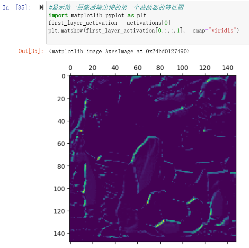
13.显示第一层激活输出特的第一个滤波器的特征图
#显示第一层激活输出特的第一个滤波器的特征图
import matplotlib.pyplot as plt
first_layer_activation = activations[0]
plt.matshow(first_layer_activation[0,:,:,1],  cmap="viridis")
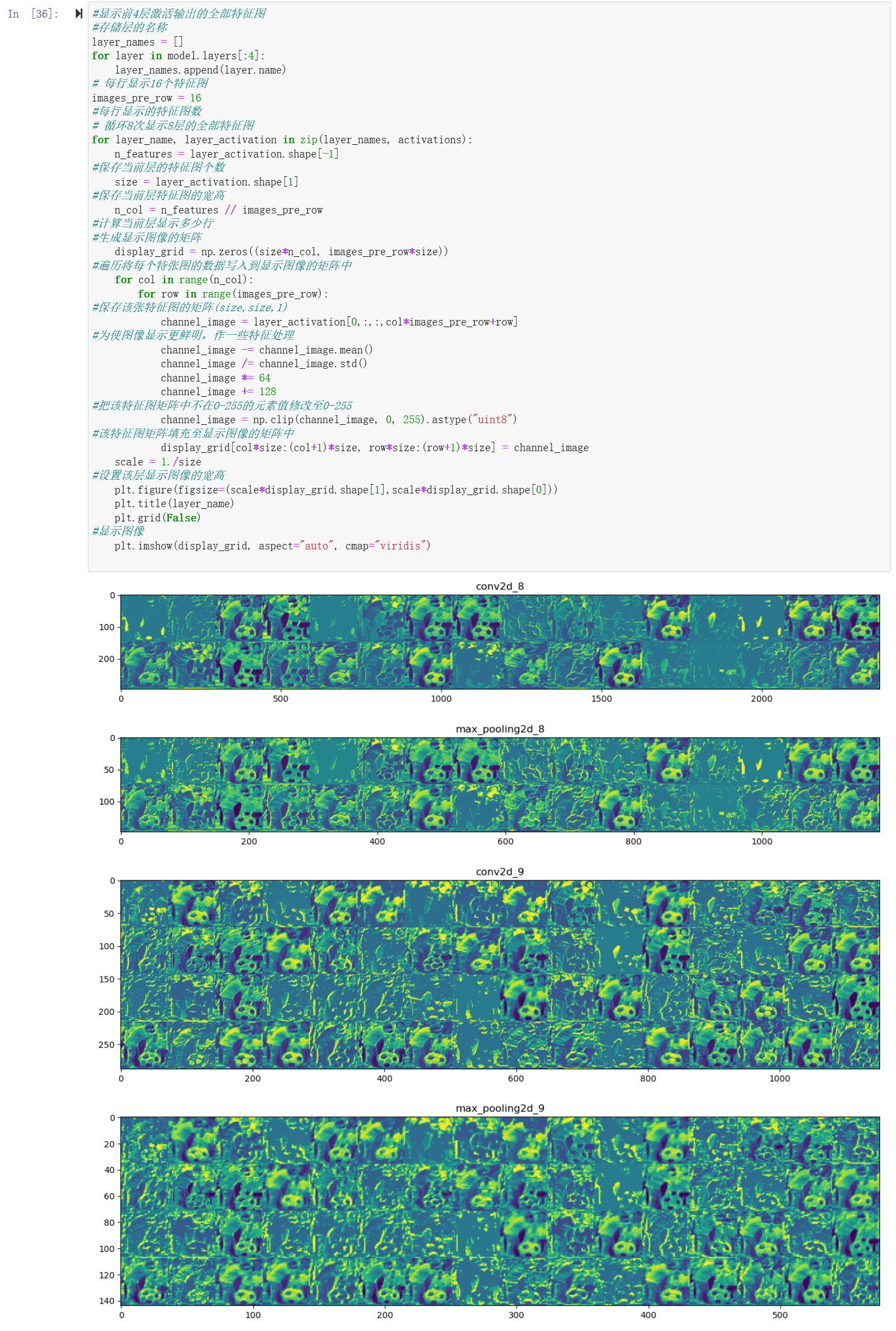
14.显示前4层激活输出的全部特征图
#显示前4层激活输出的全部特征图
#存储层的名称
layer_names = []
for layer in model.layers[:4]:
    layer_names.append(layer.name)
# 每行显示16个特征图
images_pre_row = 16
#每行显示的特征图数
# 循环8次显示8层的全部特征图
for layer_name, layer_activation in zip(layer_names, activations):
    n_features = layer_activation.shape[-1]
#保存当前层的特征图个数
    size = layer_activation.shape[1]
#保存当前层特征图的宽高
    n_col = n_features // images_pre_row
#计算当前层显示多少行
#生成显示图像的矩阵
    display_grid = np.zeros((size*n_col, images_pre_row*size))
#遍历将每个特张图的数据写入到显示图像的矩阵中
    for col in range(n_col):
        for row in range(images_pre_row):
#保存该张特征图的矩阵(size,size,1)
            channel_image = layer_activation[0,:,:,col*images_pre_row+row]
#为使图像显示更鲜明,作一些特征处理
            channel_image -= channel_image.mean()
            channel_image /= channel_image.std()
            channel_image *= 64
            channel_image += 128
#把该特征图矩阵中不在0-255的元素值修改至0-255
            channel_image = np.clip(channel_image, 0, 255).astype("uint8")
#该特征图矩阵填充至显示图像的矩阵中
            display_grid[col*size:(col+1)*size, row*size:(row+1)*size] = channel_image
    scale = 1./size
#设置该层显示图像的宽高
    plt.figure(figsize=(scale*display_grid.shape[1],scale*display_grid.shape[0]))
    plt.title(layer_name)
    plt.grid(False)
#显示图像
    plt.imshow(display_grid, aspect="auto", cmap="viridis")

15.读取图像样本,改变其尺寸

#读取图像样本,改变其尺寸
#方法1
import keras.utils as image
import numpy as np

img_path = "C:/soccer and rugby/test/soccer.2.jpg"

img = image.load_img(img_path, target_size=(150,150))
img_tensor = image.img_to_array(img)
#转换成数组
img_tensor = np.expand_dims(img_tensor, axis=0)
img_tensor /= 255.
print(img_tensor.shape)
print(img_tensor[0][0])
plt.imshow(img_tensor[0])
plt.show()
#方法2
import matplotlib.pyplot as plt
from PIL import Image
import os.path

#将图片缩小到(150,150)的大小
def convertjpg(jpgfile,outdir,width=150,height=150):
    img=Image.open(jpgfile)
    try:
        new_img=img.resize((width,height),Image.BILINEAR)
        new_img.save(os.path.join(outdir,os.path.basename(new_file)))
    except Exception as e:
        print(e)

jpgfile="C:/soccer and rugby/test/soccer.2.jpg"
new_file="C:/soccer and rugby/soccer.3.jpg"
#图像大小改变到(150,150),文件名保存
convertjpg(jpgfile,r"C:/soccer and rugby")
img_scale = plt.imread('C:/soccer and rugby/soccer.3.jpg')

#显示改变图像大小后的图片确实变到了(150,150)大小
plt.imshow(img_scale)

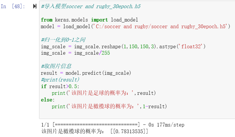
16.导入图片测试模型

#导入模型soccer and rugby_30epoch.h5

from keras.models import load_model
model = load_model('C:/soccer and rugby/soccer and rugby_30epoch.h5')
#model.summary()
img_scale = plt.imread('C:/soccer and rugby/soccer.3.jpg')
img_scale = img_scale.reshape(1,150,150,3).astype('float32')
img_scale = img_scale/255
#归一化到0-1之间

#取图片信息
result = model.predict(img_scale)

#print(result)
img_scale = plt.imread('C:/soccer and rugby/soccer.3.jpg')

#显示图片
plt.imshow(img_scale)

if result>0.5:
    print('该图片是足球的概率为:',result)
else:
    print('该图片是橄榄球的概率为:',1-result)


17.读取自定义图像文件,改尺寸后保存

#读取自定义图像文件,改尺寸后保存

import matplotlib.pyplot as plt
from PIL import Image
import os.path

#将图片缩小到(150,150)的大小
def convertjpg(jpgfile,outdir,width=150,height=150):
    img=Image.open(jpgfile)
    try:
        new_img=img.resize((width,height),Image.BILINEAR)
        new_img.save(os.path.join(outdir,os.path.basename(jpgfile)))
    except Exception as e:
        print(e)

#读取原图像
jpgfile = 'C:/soccer and rugby/sample/rugby.1.jpg'
#图像大小改变到(150,150)
convertjpg(jpgfile,"C:/A")

img_scale = plt.imread('C:/A/rugby.1.jpg')
#显示改变图像大小后的图片确实变到了(150,150)大小
plt.imshow(img_scale)


18.导入模型,测试上面保存的图片

#导入模型soccer and rugby_30epoch.h5

from keras.models import load_model
model = load_model('C:/soccer and rugby/soccer and rugby_30epoch.h5')

#归一化到0-1之间
img_scale = img_scale.reshape(1,150,150,3).astype('float32')
img_scale = img_scale/255

#取图片信息
result = model.predict(img_scale)
#print(result)
if result>0.5:
    print('该图片是足球的概率为:',result)
else:
    print('该图片是橄榄球的概率为:',1-result)
全部代码

  1 #检查一下,看看每个分组(训练 / 验证 / 测试)中分别包含多少张图像
  2 import os
  3 train_path="C:/soccer and rugby/train/"
  4 print('足球的训练集图像数量:', len(os.listdir(train_path+"soccer")))
  5 print('橄榄球的训练集图像数量:', len(os.listdir(train_path+"rugby")))
  6 print('-----------------------------------')
  7 valid_path="C:/soccer and rugby/validation/"
  8 print('足球的验证集图像数量:', len(os.listdir(valid_path+"soccer")))
  9 print('橄榄球的验证集图像数量:', len(os.listdir(valid_path+"rugby")))
 10 print('-----------------------------------')
 11 test_path="C:/soccer and rugby/test/"
 12 print('测试集图像数量:', len(os.listdir(test_path)))
 13
 14 #将足球和橄榄球的分类的小型卷积神经网络实例化
 15 from keras import layers
 16 from keras import models
 17
 18 # 使用 Sequential
 19 model = models.Sequential()
 20
 21 # 第1个 Conv2D + MaxPooling2D 组合
 22 model.add(layers.Conv2D(32, (3, 3), activation='relu',input_shape=(150, 150, 3)))
 23 model.add(layers.MaxPooling2D((2, 2)))
 24
 25 # 第2个 Conv2D + MaxPooling2D 组合
 26 model.add(layers.Conv2D(64, (3, 3), activation="relu"))
 27 model.add(layers.MaxPooling2D((2, 2)))
 28
 29 # 第3个 Conv2D + MaxPooling2D 组合
 30 model.add(layers.Conv2D(128, (3, 3), activation="relu"))
 31 model.add(layers.MaxPooling2D((2, 2)))
 32
 33 # 第4个 Conv2D + MaxPooling2D 组合
 34 model.add(layers.Conv2D(128, (3, 3), activation="relu"))
 35 model.add(layers.MaxPooling2D((2, 2)))
 36
 37 #  多维转为一维:7*7*128=6272
 38 model.add(layers.Flatten())
 39
 40 #  参数数量:6272*512+512=3211776
 41 model.add(layers.Dense(512, activation='relu'))
 42
 43 #  参数数量:512*1+1=513
 44 model.add(layers.Dense(1, activation='sigmoid'))
 45
 46 #看一下特征图的维度如何随着每层变化
 47 model.summary()
 48
 49 # 编译模型
 50 # RMSprop 优化器。因为网络最后一层是单一sigmoid单元,
 51 # 所以使用二元交叉熵作为损失函数
 52 from keras import optimizers
 53
 54 model.compile(loss='binary_crossentropy',
 55               optimizer=optimizers.RMSprop(lr=1e-4),
 56               metrics=['acc'])
 57
 58 #图像在输入神经网络之前进行数据处理,建立训练和验证数据
 59 from keras.preprocessing.image import ImageDataGenerator
 60
 61 #归一化
 62 train_datagen = ImageDataGenerator(rescale = 1./255)
 63 test_datagen = ImageDataGenerator(rescale = 1./255)
 64
 65 #指向训练集图片目录路径
 66 train_dir = 'C:/soccer and rugby/train'
 67
 68 #  输入训练图像尺寸
 69 train_generator = train_datagen.flow_from_directory(
 70     train_dir,
 71     target_size = (150,150),
 72     batch_size = 20,
 73     class_mode = 'binary')
 74
 75 #指向验证集图片目录路径
 76 validation_dir = 'C:/soccer and rugby/validation'
 77
 78 validation_generator = test_datagen.flow_from_directory(
 79     validation_dir,
 80     target_size = (150,150),
 81     batch_size = 20,
 82     class_mode = 'binary')
 83
 84 #生成器不会停止,会循环生成这些批量,所以我们就循环生成一次批量
 85 for data_batch,labels_batch in train_generator:
 86     print('图像数据组成的批量:',data_batch.shape)
 87     print('二进制标签组成的批量:',labels_batch.shape)
 88     break
 89
 90 #训练模型30轮次
 91 history = model.fit(
 92                     train_generator,
 93                     steps_per_epoch = 100,
 94 #训练30次
 95                     epochs = 30,
 96                     validation_data = validation_generator,
 97                     validation_steps = 50)
 98
 99 #将训练过程产生的数据保存为h5文件
100 from keras.models import load_model
101 model.save('C:/soccer and rugby/soccer and rugby_30epoch.h5')
102
103 #如何打开.h5文件
104 from keras.models import load_model
105 from keras import layers
106 from keras import models
107
108 model=load_model('C:/soccer and rugby/soccer and rugby_30epoch.h5')
109
110 #查看验证集的损失和准确率
111 validation_loss, validation_accuracy = model.evaluate(validation_generator)
112 print(f"Validation Loss: {validation_loss:.4f}")
113 print(f"Validation Accuracy: {validation_accuracy:.4f}")
114
115 #绘制训练过程中的损失曲线和精度曲线
116 import matplotlib.pyplot as plt
117
118 acc = history.history['acc']
119 loss =history.history['loss']
120
121 epochs = range(1,len(acc) + 1)
122
123 plt.plot(epochs,acc,'bo',label='Training acc')
124 plt.plot(epochs,loss,'b',label='loss')
125 plt.title('Training and validation accuracy')
126 plt.legend()
127
128 #绘制训练过程中的损失曲线
129 import matplotlib.pyplot as plt
130
131 loss =history.history['loss']
132 epochs = range(1,len(acc) + 1)
133 plt.plot(epochs,loss,'b',label='loss')
134 plt.title('loss')
135 plt.legend()
136
137 #绘制训练过程中精度曲线
138 import matplotlib.pyplot as plt
139 acc = history.history['acc']
140 epochs = range(1,len(acc) + 1)
141
142 plt.plot(epochs,acc,'bo',label='Training acc')
143 plt.title(' accuracy')
144 plt.legend()
145
146 #从测试集中读取一条样本
147 img_path = "C:/soccer and rugby/train/soccer/soccer.1125.jpg"
148
149 import keras.utils as image
150 import numpy as np
151
152 img = image.load_img(img_path, target_size=(150,150))
153 img_tensor = image.img_to_array(img)
154 img_tensor = np.expand_dims(img_tensor, axis=0)
155 img_tensor /= 255
156 print(img_tensor.shape)
157
158 #显示样本
159 import matplotlib.pyplot as plt
160 plt.imshow(img_tensor[0])
161 plt.show()
162
163 #建立模型,输入为原图像,输出为原模型的前8层的激活输出的特征图
164 from keras import models
165
166 layer_outputs = [layer.output for layer in model.layers[:8]]
167 activation_model = models.Model(inputs=model.input, outputs=layer_outputs)
168
169 #获得改样本的特征图
170 activations = activation_model.predict(img_tensor)
171
172 #显示第一层激活输出特的第一个滤波器的特征图
173 import matplotlib.pyplot as plt
174 first_layer_activation = activations[0]
175 plt.matshow(first_layer_activation[0,:,:,1],  cmap="viridis")
176
177 #显示前4层激活输出的全部特征图
178 #存储层的名称
179 layer_names = []
180 for layer in model.layers[:4]:
181     layer_names.append(layer.name)
182 # 每行显示16个特征图
183 images_pre_row = 16
184 #每行显示的特征图数
185 # 循环8次显示8层的全部特征图
186 for layer_name, layer_activation in zip(layer_names, activations):
187     n_features = layer_activation.shape[-1]
188 #保存当前层的特征图个数
189     size = layer_activation.shape[1]
190 #保存当前层特征图的宽高
191     n_col = n_features // images_pre_row
192 #计算当前层显示多少行
193 #生成显示图像的矩阵
194     display_grid = np.zeros((size*n_col, images_pre_row*size))
195 #遍历将每个特张图的数据写入到显示图像的矩阵中
196     for col in range(n_col):
197         for row in range(images_pre_row):
198 #保存该张特征图的矩阵(size,size,1)
199             channel_image = layer_activation[0,:,:,col*images_pre_row+row]
200 #为使图像显示更鲜明,作一些特征处理
201             channel_image -= channel_image.mean()
202             channel_image /= channel_image.std()
203             channel_image *= 64
204             channel_image += 128
205 #把该特征图矩阵中不在0-255的元素值修改至0-255
206             channel_image = np.clip(channel_image, 0, 255).astype("uint8")
207 #该特征图矩阵填充至显示图像的矩阵中
208             display_grid[col*size:(col+1)*size, row*size:(row+1)*size] = channel_image
209     scale = 1./size
210 #设置该层显示图像的宽高
211     plt.figure(figsize=(scale*display_grid.shape[1],scale*display_grid.shape[0]))
212     plt.title(layer_name)
213     plt.grid(False)
214 #显示图像
215     plt.imshow(display_grid, aspect="auto", cmap="viridis")
216
217 #读取图像样本,改变其尺寸
218 #方法1
219 import keras.utils as image
220 import numpy as np
221
222 img_path = "C:/soccer and rugby/test/soccer.2.jpg"
223
224 img = image.load_img(img_path, target_size=(150,150))
225 img_tensor = image.img_to_array(img)
226 #转换成数组
227 img_tensor = np.expand_dims(img_tensor, axis=0)
228 img_tensor /= 255.
229 print(img_tensor.shape)
230 print(img_tensor[0][0])
231 plt.imshow(img_tensor[0])
232 plt.show()
233
234 #方法2
235 import matplotlib.pyplot as plt
236 from PIL import Image
237 import os.path
238
239 #将图片缩小到(150,150)的大小
240 def convertjpg(jpgfile,outdir,width=150,height=150):
241     img=Image.open(jpgfile)
242     try:
243         new_img=img.resize((width,height),Image.BILINEAR)
244         new_img.save(os.path.join(outdir,os.path.basename(new_file)))
245     except Exception as e:
246         print(e)
247
248 jpgfile="C:/soccer and rugby/test/soccer.2.jpg"
249 new_file="C:/soccer and rugby/soccer.3.jpg"
250 #图像大小改变到(150,150),文件名保存
251 convertjpg(jpgfile,r"C:/soccer and rugby")
252 img_scale = plt.imread('C:/soccer and rugby/soccer.3.jpg')
253
254 #显示改变图像大小后的图片确实变到了(150,150)大小
255 plt.imshow(img_scale)
256
257 #导入模型soccer and rugby_30epoch.h5
258
259 from keras.models import load_model
260 model = load_model('C:/soccer and rugby/soccer and rugby_30epoch.h5')
261 #model.summary()
262 img_scale = plt.imread('C:/soccer and rugby/soccer.3.jpg')
263 img_scale = img_scale.reshape(1,150,150,3).astype('float32')
264 img_scale = img_scale/255
265 #归一化到0-1之间
266
267 #取图片信息
268 result = model.predict(img_scale)
269
270 #print(result)
271 img_scale = plt.imread('C:/soccer and rugby/soccer.3.jpg')
272
273 #显示图片
274 plt.imshow(img_scale)
275
276 if result>0.5:
277     print('该图片是足球的概率为:',result)
278 else:
279     print('该图片是橄榄球的概率为:',1-result)
280
281 #读取自定义图像文件,改尺寸后保存
282
283 import matplotlib.pyplot as plt
284 from PIL import Image
285 import os.path
286
287 #将图片缩小到(150,150)的大小
288 def convertjpg(jpgfile,outdir,width=150,height=150):
289     img=Image.open(jpgfile)
290     try:
291         new_img=img.resize((width,height),Image.BILINEAR)
292         new_img.save(os.path.join(outdir,os.path.basename(jpgfile)))
293     except Exception as e:
294         print(e)
295
296 #读取原图像
297 jpgfile = 'C:/soccer and rugby/sample/rugby.1.jpg'
298 #图像大小改变到(150,150)
299 convertjpg(jpgfile,"C:/A")
300
301 img_scale = plt.imread('C:/A/rugby.1.jpg')
302 #显示改变图像大小后的图片确实变到了(150,150)大小
303 plt.imshow(img_scale)
304
305 #导入模型soccer and rugby_30epoch.h5
306
307 from keras.models import load_model
308 model = load_model('C:/soccer and rugby/soccer and rugby_30epoch.h5')
309
310 #归一化到0-1之间
311 img_scale = img_scale.reshape(1,150,150,3).astype('float32')
312 img_scale = img_scale/255
313
314 #取图片信息
315 result = model.predict(img_scale)
316 #print(result)
317 if result>0.5:
318     print('该图片是足球的概率为:',result)
319 else:
320     print('该图片是橄榄球的概率为:',1-result)
四、总结
本次的程序设计主要内容是机器学习——识别足球和橄榄球,通过本次课程设计,我对机器学习有了进一步的认识与了解,但在编写运行代码的过程中,也经常会遇到报错,通过一次次的修正,代码的编写也更快了。我切身感受到,在学习python的过程中,实践尤其的重要,只有通过亲自操作,才会发现自己学习过程中的不足之处,这对于我学习python,非常的有帮助。这次程序设计中,模型训练达到了预期的效果,但是发现自己刚开始对程序设计完整的构思并没有很清晰,所以花费了很多时间改正,通过这次的学习,我也将对于程序设计的构思有了进一步的完善。