第七章 图像分割

第七章 图像分割

• 点、线和边缘检测
  
  • 点检测
  • 线检测
  • 使用函数edge检测边缘
• 使用霍夫变换进行行线检测
  
  • 背景知识
  • 工具箱霍夫函数
• 阈值处理
  
  • 基础知识
  • 基本的全局阈值处理
  • 使用Otsu方法进行最佳全局阈值处理
  • 使用图像平滑改进全局阈值处理
  • 使用边缘改进全局阈值处理
  • 基于局部统计的可变阈值处理
  • 使用移动平均的图像阈值处理

一.点、线和边缘检测

在检测三种类型的灰度不连续性时常使用imfilter描述的方法，对图像应用模板。

点检测

• imfilter函数

在之前的学习中已经涉及到了这一函数，当时使用它进行线性空间滤波操作，现在用来实现点的检测。

==在滤波操作中使用tofloat防止数值的过早截断。==

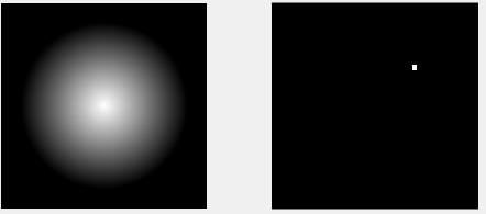
>> w = [-1 -1 -1; -1 8 -1; -1 -1 -1];
>> f = Fig1002;
>> g = abs(imfilter(tofloat(f), w));
>> T = max(g(:));
>> g = g >= T;
>> subplot(121), imshow(f);
>> subplot(122), imshow(g);

实际上在东北方向检测到了该点，放大后图像如下图，可以明显看出该点。

• ordfilt2函数

非线性空间滤波器操作过程中，是使用了ordfilt2函数，也同样可以进行点检测。

>> m = 5; n = m;
>> g = ordfilt2(f, m*n, ones(m, n)) - ordfilt2(f, 1, ones(m, n));
>> T = max(g(:));
>> g = g>= T;
>> imshow(g);

很明显可以看到东北方向的白点，和上面结果是相同的。（红色圈圈出）

线检测

线检测一般应用基础的线检测模板，在水平、垂直、+45度和-45度这四种基础模板中进行选择。

模板的优先方向一般会形成最强响应。

>> f = Fig1004;
>> w = [2 -1 -1; -1 2 -1; -1 -1 2];
>> g = imfilter(tofloat(f), w);
>> subplot(121), imshow(f), title('原图');
>> subplot(122), imshow(g, []), title('w过滤器过滤后');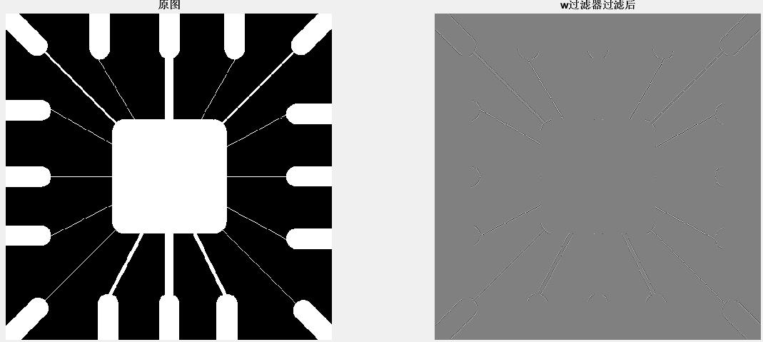

放大左上角和右下角的图像

>> gtop = g(1: 180, 1:180);
>> gtop = pixeldup(gtop, 4);
>> subplot(121), imshow(gtop, []), title('左上角');
>> gbot = g(end - 179:end, end - 179:end);
>> gbot = pixeldup(gbot, 4);
>> subplot(122), imshow(gbot, []), title('右下角');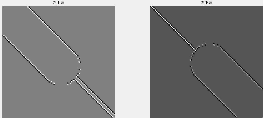

在图中进行点检测

>> g = imfilter(tofloat(f), w);
>> g = abs(g);
>> subplot(121), imshow(g, []), title('w滤波器过滤后图像的绝对值');
>> T = max(g(:));
>> g = g>= T;
>> subplot(122), imshow(g), title('满足g>=T的点');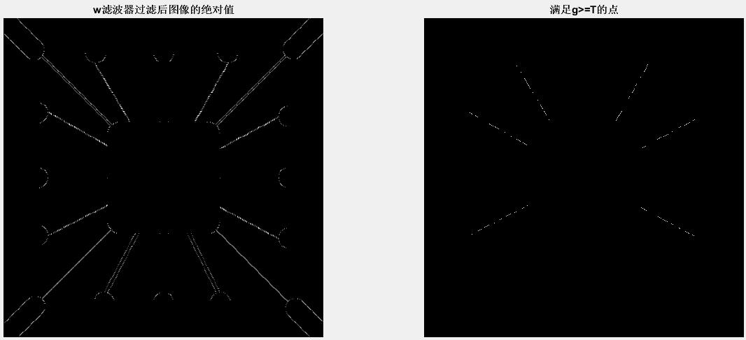

使用函数edge检测边缘

边缘检测基本思想有两个准则：（一）寻找灰度的一阶导数的幅度大于某个指定阈值的位置。（二）寻找灰度的二阶导数有零交叉的位置。

函数edge

edge提供了边缘检测器

[g, t] = edge(f, ‘method’, parameters)

method表示边缘检测器的模式，parameters表示其他参数。

• Sobel边缘检测器

[g, t] = edge(f, ‘sobel’, T, dir)

dir表示方向：’horizontal’(水平的), ‘vertical’(垂直的), ‘both’(默认)。T表示一个指定的阈值。

>> f = Fig1006;
>> [gv, t] = edge(f, 'sobel', 'vertical');
>> t

t =

    0.0516
>> subplot(231), imshow(f), title('原图');
>> subplot(232), imshow(gv), title('sobel垂直边缘');
>> gv = edge(f, 'sobel', 0.15, 'vertical');
>> subplot(233), imshow(gv), title('阈值0.15');
>> gboth = edge(f, 'sobel', 0.15);
>> subplot(234), imshow(gboth), title('检测整体边缘，阈值0.15');
>> wneg45 = [-2 -1 0; -1 0 1; 0 1 2];
>> gneg45 = imfilter(tofloat(f), wneg45, 'replicate');
>> T = 0.3 * max(abs(gneg45(:)));
>> gneg45 = gneg45 >= T;
>> subplot(235), imshow(gneg45), title('-45度最强边缘');
>> wpos45 = [0 1 2; -1 0 1; -2 -1 0];
>> gpos45 = imfilter(tofloat(f), wpos45, 'replicate');
>> T = 0.3*max(abs(gpos45(:)));
>> gpos45 = gpos45 >= T;
>> subplot(236), imshow(gpos45), title('+45度最强边缘');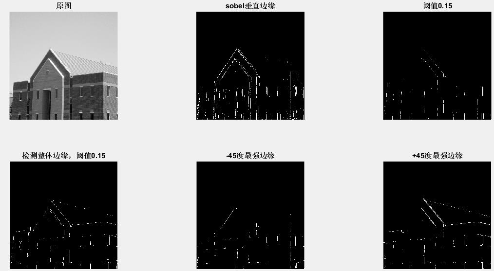

• Prewitt边缘检测器
  

  [g, t] = edge(f, ‘prewitt’, T, dir)

缺点：噪声稍微大一些。

• Roberts边缘检测器
  

  [g, t] = edge(f, ‘roberts’ ,T, dir)

功能有限但是优点在于简单和速度。

• LoG检测器
  

  [g, t] = edge(f, ‘log’, T, sigma)

sigma表示标准差，默认值为2.

• 零交叉检测器

  [g, t] = edge(f, ‘zerocross’, T, H)

• Canny边缘检测器

这是edge中最强大的检测器，在我看来它总结了LoG和Sobel的方法，使其功能更强大。

[g, t] = edge(f, ‘canny’, T, sigma)

sigma的默认值为1。T = [T1, T2]是两个阈值的向量。

• 举例比较Sobel、LoG和Canny边缘检测器

>> g = tofloat(f);
>> [gSobel_default, ts] = edge(g, 'sobel');
>> [gLoG_default, tlog] = edge(g, 'log');
>> [gCanny_default, tc] = edge(g, 'canny');
>> gSobel_best = edge(g, 'sobel', 0.05);
>> gLoG_best = edge(g, 'log', 0.003, 2.25);
>> gCanny_best = edge(g, 'canny', [0.04, 0.10], 1.5);
>> subplot(231), imshow(gSobel_default), title('Sobel默认');
>> subplot(232), imshow(gLoG_default), title('LoG默认');
>> subplot(233), imshow(gCanny_default), title('Canny默认');
>> ts

ts =

    0.0738

>> tlog

tlog =

    0.0020

>> tc

tc =

    0.0188    0.0469
>> subplot(234), imshow(gSobel_best), title('Sobel阈值0.05');
>> subplot(235), imshow(gLoG_best), title('Log阈值0.003,标准差2.25');
>> subplot(236), imshow(gCanny_best), title('Canny阈值向量[0.004, 0.10],标准差1.5');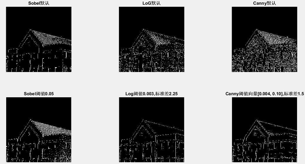

Canny的结果要远远好于两种，这也就是上面提到的是edge中最强大的边缘检测器。

• 关于阈值处理的一些问题

在没学到7.3之前对于阈值也有很多疑惑，所以基于上面的比较，我进行了一些实验操作，来理解阈值对于图像处理的实际情况。

>> gs = edge(g, 'sobel', 0.0134);
>> figure, subplot(121), imshow(gs), title('阈值0.0134（小）');
>> gs = edge(g, 'sobel', 0.09);
>> subplot(122), imshow(gs), title('阈值0.09（大）');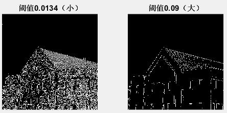

很明显sobel当==比默认阈值小==的时候，图像边缘显示==更密集==；当==比默认阈值大==的时候，图像显示的比默认时显示的==更少，更稀疏==。

经过实践比对，LoG和Canny也同样。

• 关于标准差的一些问题

在LoG检测器和Canny检测器中都有标准差的存在，标准差更倾向于对于图像进行平滑处理时所需要的数据。

以Canny为例

>> gc = edge(g, 'canny', [0.01, 0.03]);
>> figure, subplot(121), imshow(gCanny_default), title('默认Canny');
>> subplot(122), imshow(gc), title('阈值整体变小，标准差默认');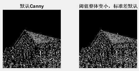

>> gc = edge(g, 'canny', tc, 2.5);
>> subplot(121), imshow(gCanny_default), title('默认Canny');
>> subplot(122), imshow(gc), title('阈值默认，标准差变2.5（大）');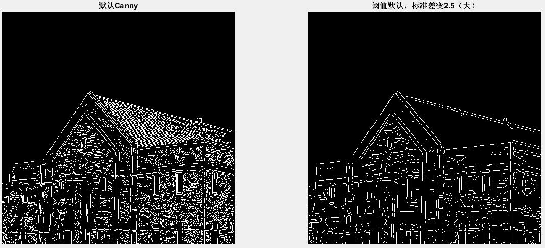

线条变得更稀疏。

二.使用霍夫变换进行线检测

背景知识

在执行边缘检测算法后，通常会使用连接过程来把边缘像素组装成有意义的边缘，连接图像中线段的一种方式就是霍夫变换。

在霍夫变换中，参数空间交点的横纵坐标用来表示平面直线的斜率和截距。

工具箱霍夫函数

• 函数hough

[H, theta, rho] = hough(f)

H是霍夫变换矩阵，theta和rho是向量。

>> f = zeros(101, 101);
>> f(1, 1) = 1;
>> f(101, 1) = 1;
>> f(1, 101) = 1;
>> f(101, 101) = 1;
>> f(51, 51) = 1;
>> H = hough(f);
>> subplot(121), imshow(f),title('f');
>> subplot(122), imshow(H, []),title('hough变换后');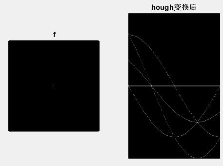

显示标上值之后的结果

>> [H, theta, rho] = hough(f);
>> imshow(H, [], 'XData', theta, 'YData', rho, 'InitialMagnification', 'fit');
>> axis on, axis normal
>> xlabel('\theta'), ylabel('\rho')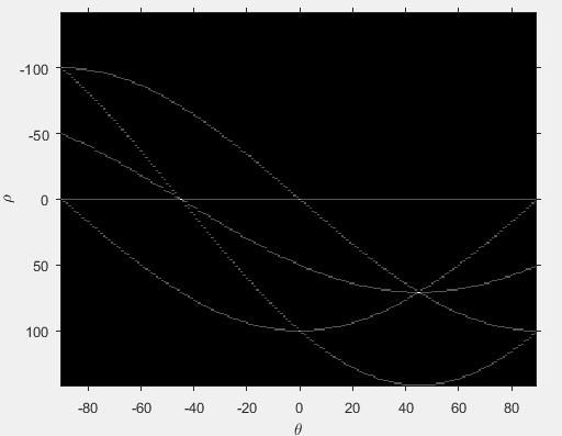

• 函数houghpeaks

peaks = houghpeaks(H, NumPeaks)

NumPeaks表示要找到指定数量的封装。

• 函数houghlines

lines = houghlines(f, theta, rho, peaks)

该结构的每个元素识别一条线，并有==如下字段==：

1.point1，一个两元素向量[r1, c1]，它指定线段终点的行、列坐标。

2.point2，一个两元素向量[r2, c2]，它指定线段其他终点的行、列坐标。

3.theta，与线相关的活法变换容器的角度（单位为度）。

4.rho，与线相关的霍夫变换容器的rho轴的位置。

• 使用霍夫变换做检测和连接

>> f = gCanny_best;
>> [H, theta, rho] = hough(f, 'ThetaResolution', 0.2);
>> imshow(H, [], 'XData', theta, 'YData', rho, 'InitialMagnification', 'fit');
>> axis on, axis normal
>> xlabel('\theta'), ylabel('\rho')
>> peaks = houghpeaks(H, 5);
>> hold on
>> plot(theta(peaks(:, 2)), rho(peaks(:, 1)),...
'linestyle', 'none', 'marker', 's', 'color', 'w')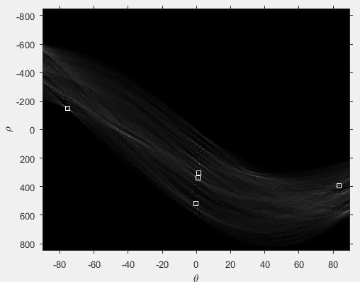

>> lines = houghlines(f, theta, rho, peaks);
>> figure, imshow(f), hold on
>> for k = 1:length(lines)
xy = [lines(k).point1; lines(k).point2];
plot(xy(:, 1), xy(:, 2), 'LineWidth', 4, 'Color', [.8 .8 .8]);
end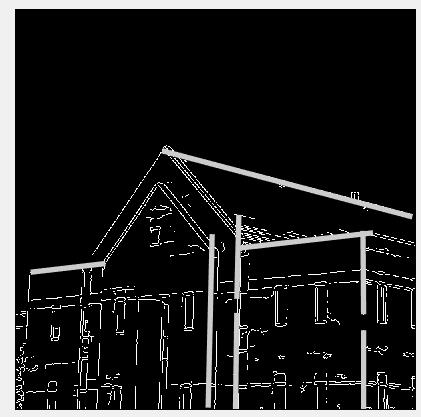

• 练习
  找出最长的线

%霍夫变换
>> gc = edge(f, 'Canny');
>> gc = tofloat(gc);
>> [H, theta, rho] = hough(gc);
>> imshow(H, [], 'XData', theta, 'YData', rho, 'InitialMagnification', 'fit');
>> axis on, axis normal
>> xlabel('\theta'), ylabel('\rho')
>> hold on

%霍夫变换线的检测
>> peaks = houghpeaks(H, 5);
>> plot(theta(peaks(:, 2)), rho(peaks(:, 1)), 'linestyle', 'none', 'marker', 's', 'color', 'y');
>> lines = houghlines(gc, theta, rho, peaks);
>> figure, imshow(gc), hold on
%最长线
>> maxline = 0;
>> for k = 1:length(lines)
xy = [lines(k).point1; lines(k).point2];
len = max(svd(lines(k).point1 - lines(k).point2));
if len > maxline
maxline = len;
xylong = xy;
end
end
>> plot(xylong(:, 1), xylong(:, 2), 'LineWidth',2,'Color','red');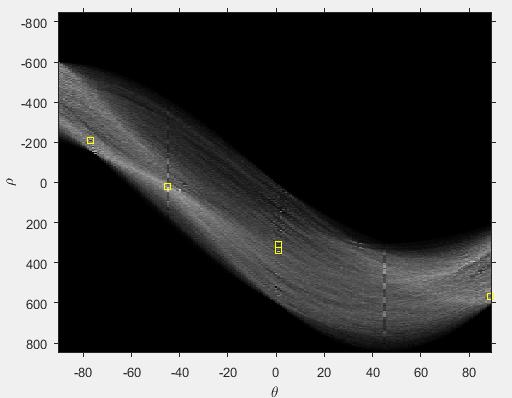

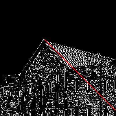
==svd是一种正交矩阵分解，求出向量的距离的最大值，即是最长的线段==

三.阈值处理

基础知识

我理解的阈值就是图像中的临界值，也就是界限。

全局阈值处理：T是一个使用于整个图像的常数。

可变阈值处理：T在一幅图像上变化。（局部阈值处理或区域阈值处理也用于表示这样一种可变阈值处理。）

基本的全局阈值处理

g = im2bw(f, T/ben)

im2bw函数分割图像

>> f = Fig1013;
>> count = 0;
>> T = mean2(f);
>> done = false;
>> while ~done
count = count + 1;
g = f > T;
Tnext = 0.5 * (mean(f(g)) + mean(f(~g)));
done = abs(T - Tnext) < 0.5;
T = Tnext;
end
>> count

count =

     2

>> T

T =

  125.3860

>> g = im2bw(f, T/255);
>> subplot(131), imshow(f), title('原图');
>> subplot(132), imhist(f), title('直方图');
>> subplot(133), imshow(g), title('全局阈值');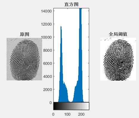

这是处理全局阈值的基本方法。

代码中mean()表示求列或行的平均数，mean2()表示相当于对整个矩阵求像素平均值。

使用Otsu方法进行最佳全局阈值处理

• 函数graythresh

[T, SM] = graythresh(f)

T是产生的阈值，它被归一化到区间[0, 1]。

>> f = Fig1014;
>> [T, SM] = graythresh(f)

T =

    0.7098


SM =

    0.4662

>> T * 255

ans =

   181
>> subplot(221), imshow(f), title('原图');
>> subplot(222), imhist(f), title('直方图');
>> g = im2bw(f, T);
>> subplot(224), imshow(g), title('Otsu全局阈值处理');
>> count = 0;
T = mean2(f);
done = false;
while ~done
count = count + 1;
g = f > T;
Tnext = 0.5 * (mean(f(g)) + mean(f(~g)));
done = abs(T - Tnext) < 0.5;
T = Tnext;
end
>> g = im2bw(f, T/255);
>> subplot(223), imshow(g), title('基本全局阈值处理');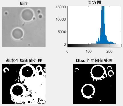

可以明显得看出基本方法处理的图像比较粗糙，有很大一部分处理不当，与原图相背离，Otsu将图像的大致轮廓都显示出来。

使用图像平滑改进全局阈值处理

噪声会把一些简单的阈值处理问题变得不能解决，所以我们对图像进行平滑处理来减少噪声的影响。

复习了之前的内容，平滑处理需要函数special来形成滤波算子，在使用imfilter函数进行图像平滑。

>> f = Fig1015;
>> fn = imnoise(f, 'gaussian', 0, 0.038);
>> subplot(231), imshow(fn), title('带噪图像');
>> subplot(232), imhist(fn), title('带噪图像直方图');
>> T = graythresh(fn);
>> g = im2bw(fn, T);
>> subplot(233), imshow(g), title('Ostu阈值处理');
>> w = fspecial('average', 5);
>> gn = imfilter(fn, w, 'replicate');
>> subplot(234), imshow(gn), title('平滑');
>> subplot(235), imhist(gn), title('平滑直方图');
>> T = graythresh(gn);
>> g1 = im2bw(gn, T);
>> subplot(236), imshow(g1), title('平滑后Ostu阈值处理');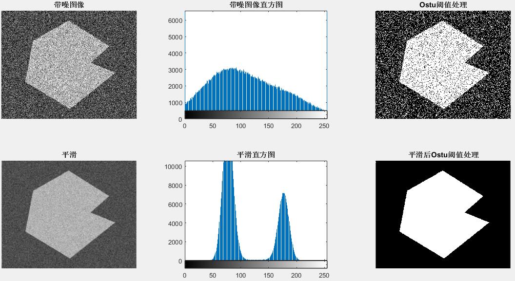

使用边缘改进全局阈值处理

之前的方法是假设物体和背景之间的边缘已知。寻找一个分界线正是分割要做的，我们可以通过两种方法实现：计算梯度或拉普拉斯算子的绝对值。

• 基于梯度

>> f = Fig1016;
>> g = tofloat(f);
>> sx = fspecial('sobel');
>> sy = sx';
>> gx = imfilter(g, sx, 'replicate');
>> gy = imfilter(g, sy, 'replicate');
>> grad = sqrt(gx.*gx + gy.*gy);
>> grad = grad / max(grad(:));
>> h = imhist(grad);
>> subplot(231), imshow(f), title('原图');
>> subplot(232), imhist(f), title('直方图');
>> Q = percentile2i(h, 0.99);
>> markerImage = grad > Q;
>> fp = g.*markerImage;
>> subplot(233), imshow(markerImage), title('阈值处理后梯度图像');
>> subplot(234), imshow(fp), title('原图像与梯度图像乘积');
>> hp = imhist(fp);
>> hp(1) = 0;
>> T = otsuthresh(hp);
>> T * (numel(hp) - 1)

ans =

   138

>> g = im2bw(g, T);
>> subplot(235), imshow(g), title('Ostu阈值分割');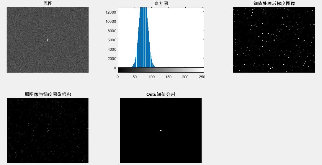

• 拉普拉斯算子

>> f = Fig1017;
>> g = tofloat(f);
>> subplot(231), imshow(g), title('原图');
>> subplot(232), imhist(g), title('直方图');
>> [T, SMf] = graythresh(g);
>> gf = im2bw(g, T);
>> subplot(233), imshow(gf), title('Ostu阈值处理');
>> w = [-1 -1 -1; -1 8 -1; -1 -1 -1];
>> lap = abs(imfilter(g, w, 'replicate'));
>> lap = lap / max(lap(:));
>> h = imhist(lap);
>> Q = percentile2i(h, 0.995);
>> markerImage = lap > Q;
>> fp = g .* markerImage;
>> subplot(234), imshow(fp), title('图像乘积');
>> hp = imhist(fp);
>> hp(1) = 0;
>> subplot(235), bar(hp, 0), title('非0像素直方图');
>> T = otsuthresh(hp);
>> g = im2bw(g, T);
>> subplot(235), imshow(g);

基于局部统计的可变阈值处理

自定义函数localthresh进行局部操作

>> f = Fig1018;
>> g = tofloat(f);
>> [T] = graythresh(g);
>> g1 = im2bw(g, T);
>> subplot(121), imshow(g);
>> subplot(222), imshow(g1), title('Otsu阈值处理');
>> g2 = localthresh(g, ones(3), 30, 1.5, 'global');
>> SIG = stdfilt(f, ones(3));
>> subplot(223), imshow(SIG, []), title('局部标准差');
>> subplot(224), imshow(g2), title('局部阈值处理');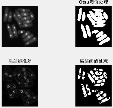

从图片中可以清晰看出局部处理和全局处理的区别，全局处理是相对于整张图像处理其中存在的图形，是整体分析；局部处理是将全局处理出来的图形再次细化，显示出其内部的结构。

使用移动平均的图形阈值处理

>> f = Fig1019;
>> T = graythresh(f);
>> g = im2bw(f, T);
>> subplot(131), imshow(f), title('原图');
>> subplot(132), imshow(g), title('Otsu阈值处理');
>> g2 = movingthresh(f, 20, 0.5);
>> subplot(133), imshow(g2), title('移动平均局部阈值处理');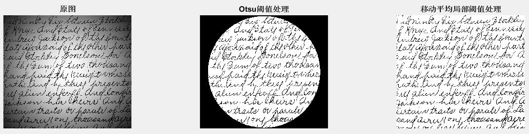

将原有图像显示不清晰的部分的遮盖物去除，全局处理后再移动平均阈值局部处理。