scikit-learn集成学习代码批注及相关练习

一、代码批注

代码来自：https://scikit-learn.org/stable/auto_examples/ensemble/plot_adaboost_twoclass.html#sphx-glr-auto-examples-ensemble-plot-adaboost-twoclass-py

import numpy as np
import matplotlib.pyplot as plt
from sklearn.ensemble import AdaBoostClassifier
from sklearn.tree import DecisionTreeClassifier
from sklearn.linear_model import LogisticRegression
from sklearn.linear_model import SGDClassifier
from sklearn.datasets import make_gaussian_quantiles
from sklearn.datasets import make_classification

# 生成数据集
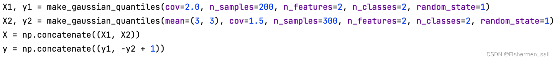
# X1, y1 = make_gaussian_quantiles(cov=2.0, n_samples=200, n_features=2, n_classes=2, random_state=1)
# X2, y2 = make_gaussian_quantiles(mean=(3, 3), cov=1.5, n_samples=300, n_features=2, n_classes=2, random_state=1)
# X = np.concatenate((X1, X2))
# y = np.concatenate((y1, -y2 + 1))
X, y = make_classification(n_samples=1000, n_features=2,  n_redundant=0, random_state=6)

# 生明AdaBoostClassifier预估器
bdt = AdaBoostClassifier(DecisionTreeClassifier(max_depth=1), algorithm="SAMME", n_estimators=3000)
# bdt = AdaBoostClassifier(SGDClassifier(loss='hinge'), algorithm="SAMME", n_estimators=1000)
# bdt = AdaBoostClassifier(LogisticRegression(), algorithm="SAMME", n_estimators=3000)
bdt.fit(X, y)

plot_colors = "br"
plot_step = 0.02
class_names = "AB"
plt.figure(figsize=(10, 5))

plt.subplot(121)
# 这里画图的方法与Knn的一样
# 画出决策边界，用不同颜色表示
x_min, x_max = X[:, 0].min() - 1, X[:, 0].max() + 1
y_min, y_max = X[:, 1].min() - 1, X[:, 1].max() + 1
# np.meshgrid：生成网格点坐标矩阵（因为pcolormesh需要这样使用）
# np.arange：起始，终点，步长
# xx,yy分别为两个特征
# 这里的意思就是为了有底色，每个x和y都都进行组合计算，算出它呢个点的底色。上面X和y相当于是训练集，这里差不多可以算作是没有结果的测试集
xx, yy = np.meshgrid(np.arange(x_min, x_max, plot_step), np.arange(y_min, y_max, plot_step))
# 用ravel()方法将数组拉成一维数组
# np.c 就是按列叠加两个矩阵，就是把两个矩阵左右组合，要求行数相等。
Z = bdt.predict(np.c_[xx.ravel(), yy.ravel()])
Z = Z.reshape(xx.shape)
# contourf：画轮廓图（与pcolormesh图形效果类似）
cs = plt.contourf(xx, yy, Z, cmap=plt.cm.Paired)
plt.axis("tight")

# 补充训练数据点
for i, n, c in zip(range(2), class_names, plot_colors):
    idx = np.where(y == i)
    plt.scatter(
        X[idx, 0],
        X[idx, 1],
        c=c,
        cmap=plt.cm.Paired,
        s=20,
        edgecolor="k",
        label="Class %s" % n,
    )
plt.xlim(x_min, x_max)
plt.ylim(y_min, y_max)
plt.legend(loc="upper right")
plt.xlabel("x")
plt.ylabel("y")
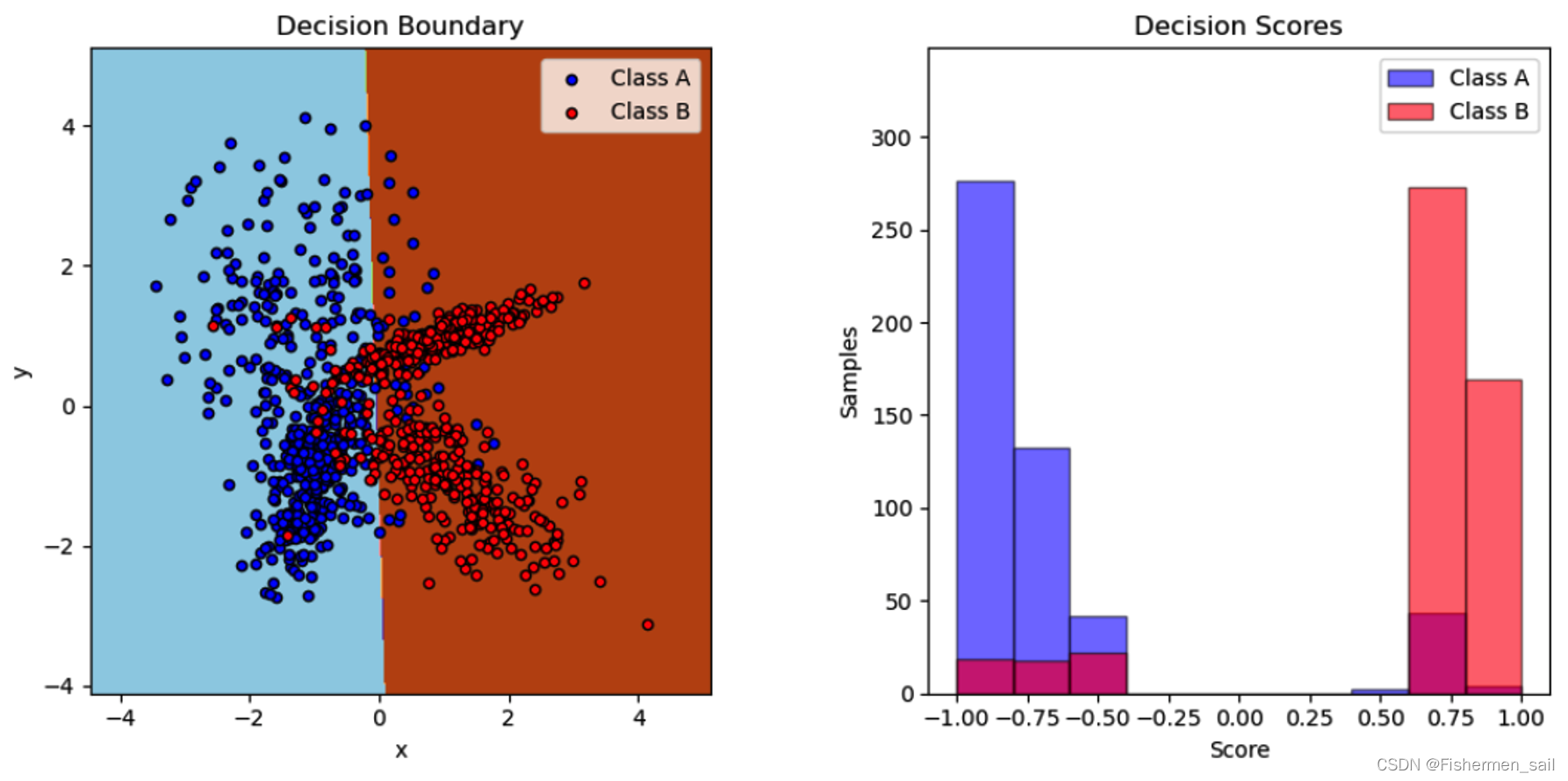
plt.title("Decision Boundary")

# 画出两类的分别决定成绩
twoclass_output = bdt.decision_function(X)
plot_range = (twoclass_output.min(), twoclass_output.max())
plt.subplot(122)
for i, n, c in zip(range(2), class_names, plot_colors):
    plt.hist(
        twoclass_output[y == i],
        bins=10,
        range=plot_range,
        facecolor=c,
        label="Class %s" % n,
        alpha=0.5,
        edgecolor="k",
    )
x1, x2, y1, y2 = plt.axis()
plt.axis((x1, x2, y1, y2 * 1.2))
plt.legend(loc="upper right")
plt.ylabel("Samples")
plt.xlabel("Score")
plt.title("Decision Scores")
plt.tight_layout()
plt.subplots_adjust(wspace=0.35)
plt.show()

二、更换机器学习数量

AdaBoostClassifier的原理是先训练一个弱学习器模型，然后对他的结果进行评估，对于这个模型中做对的问题，我们将减少它的注意力，对于做错的问题我们将增大对他的注意力，从而在后续的新模型中，更专注克服前一个模型所不能解决的困难点，最后，当我们把所有模型整合在一起，构成一个大的框架，大框架中有处理简单问题的模型，也有处理困难问题的模型，使大框架的整体性能有所提高。
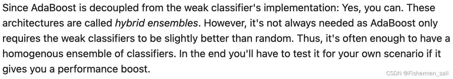
根据它的原理，在任务中要修改基学习器的数量，起初我以为是在AdaBoostClassifier的base_estimator放入更多模型，像Staking一样，但AdaBoostClassifier并不能这样做，在Stack Overflow中有网友也回答道，理论上可以的，但AdaBoostClassifier仅仅要求弱学习器比随机的好一些，因此它经常只是用同一种的分类器。
在这里插入图片描述
而任务中修改基学习器的数量因该指的是修改n_estimators的大小，它是弱学习器的最大迭代次数，也可以说是最大的弱学习器的个数。通过下图的测试如果太小，容易欠拟合，分类面比较规则，如果太大，容易过拟合，1000左右比较为宜。
在这里插入图片描述

三、更换机器学习器类型

base_estimator：默认为DecisionTreeClassifier。理论上可以选择任何一个分类或者回归学习器，不过需要支持样本权重，比如说Knn，MLP就不支持，会报“xxx doesn’t support sample_weight.”。我之后选择了逻辑回归模型，但一直报“BaseClassifier in AdaBoostClassifier ensemble is worse than random, ensemble can not be fit.”网络上也几乎没有对这个原因的解释。不仅仅是逻辑回归，SGD也不行，经过不断尝试，发现如果将下图生成数据的方式改为make_classification的方式，代码将成功执行，原因尚不清楚。
在这里插入图片描述