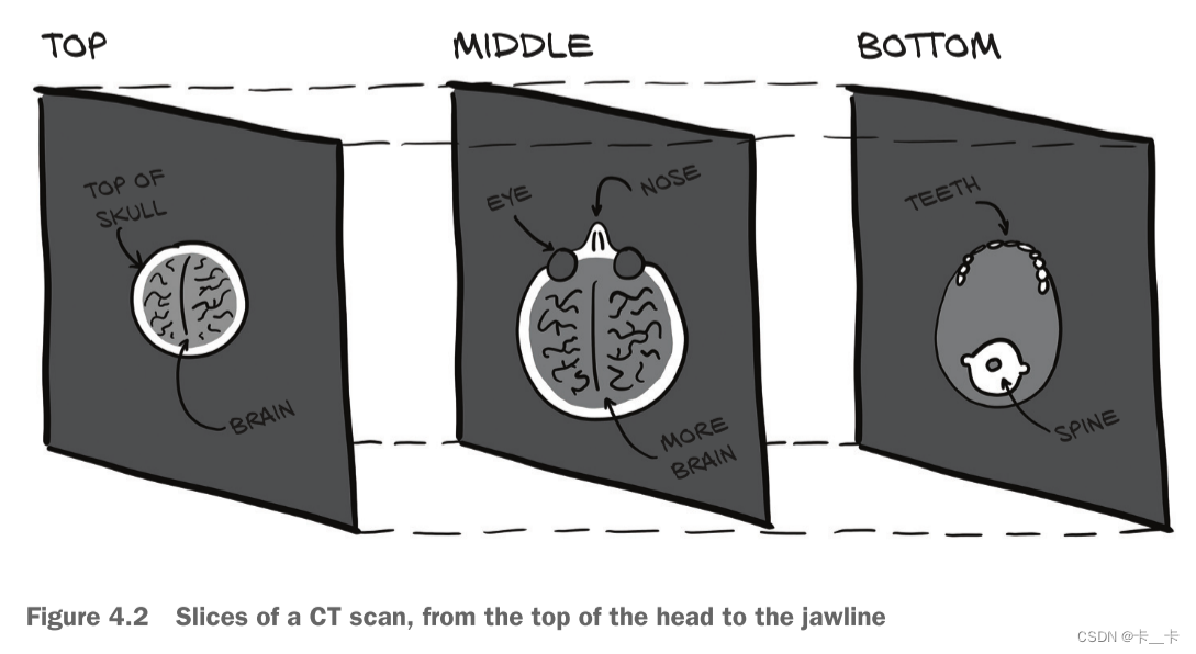
By stacking individual 2D slices into a 3D tensor, we can build volumetric data representing the 3D anatomy of a
subject. We just have an extra dimension, depth, after the channel dimension, leading to a 5D tensor of shape N × C × D × H × W.
N 表示样本(图片)的数量
C 表示特征通道的数量
D 表示深度维度的大小(例如,对于三维图像,表示图像的深度)
H 表示图像的高度
W 表示图像的宽度
Let’s load a sample CT scan using the volread function in the imageio module, which takes a directory as an argument and assembles all Digital Imaging and Communications in Medicine (DICOM) files in a series in a NumPy 3D array.
import imageio.v2 as imageio
dir_path = "D:/Deep-Learning/资料/dlwpt-code-master/data/p1ch4/volumetric-dicom/2-LUNG 3.0  B70f-04083"
# volread从文件中读取三维体积数据,返回结果为NumPy数组
vol_arr = imageio.volread(dir_path, 'DICOM')  # DICOM表示要使用的解码器格式,以确保正确解析DICOM文件
vol_arr.shape  # 结果的99表示该三维图像是由99张2维图像从bottom到top叠加得到的

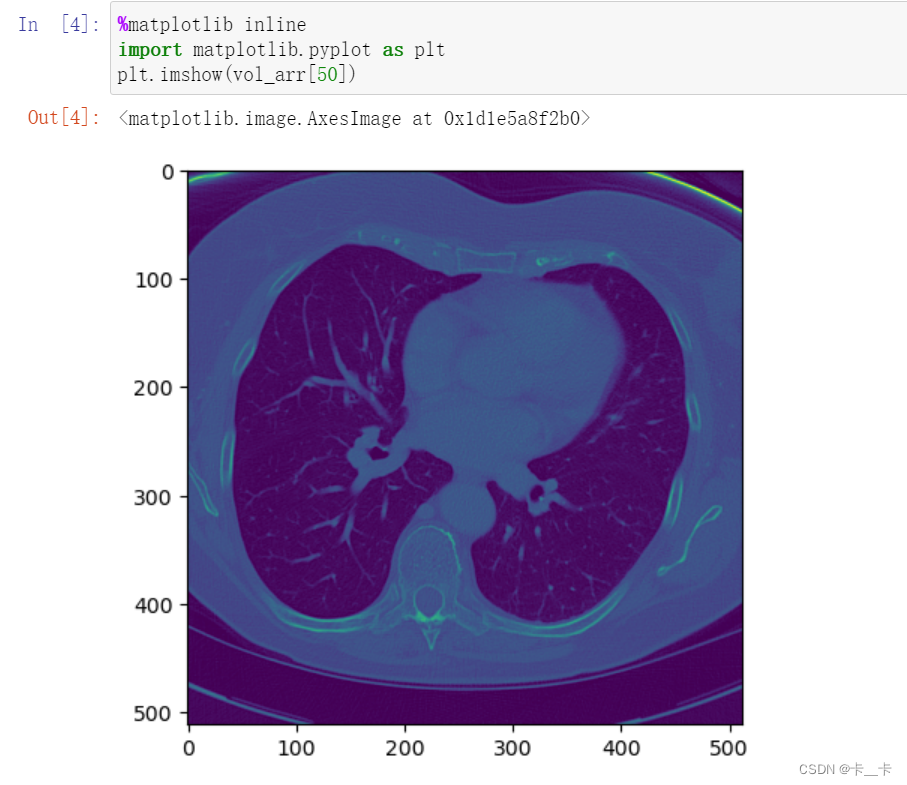
我们可以使用以下代码打印其中的某张图片,例如第50张
%matplotlib inline
import matplotlib.pyplot as plt
plt.imshow(vol_arr[50])
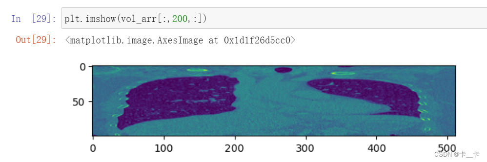
纵切面
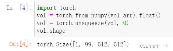
The layout is different from what PyTorch expects, due to having no channel information. So we’ll have to make room for the channel dimension using unsqueeze:
import torch
vol = torch.from_numpy(vol_arr).float()
vol = torch.unsqueeze(vol, 0)
vol.shape
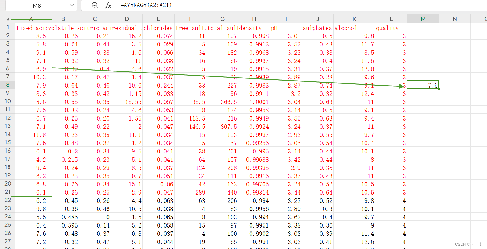
The simplest form of data we’ll encounter on a machine learning job is sitting in a spreadsheet, CSV file, or database. Whatever the medium, it’s a table containing one row per sample (or record), where columns contain one piece of information about our sample.
Columns may contain numerical values, like temperatures at specific locations; or labels, like a string expressing an attribute of the sample, like “blue.” Therefore, tabular data is typically not homogeneous: different columns don’t have the same type. We might have a column showing the weight of apples and another encoding their color in a label.

PyTorch tensors, are homogeneous. Information in PyTorch is typically encoded as a number, typically floating-point (though integer types and Boolean are supported as well).
Our first job as deep learning practitioners is to encode heterogeneous, real-world data into a tensor of floating-point numbers, ready for consumption by a neural network.
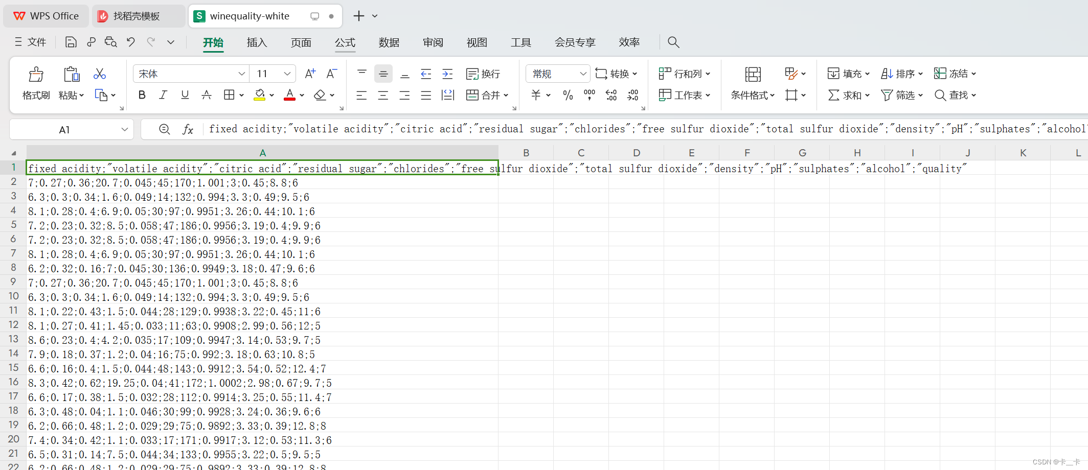
The first 11 columns contain values of chemical variables, and the last column contains the sensory quality score from 0 (very bad) to 10 (excellent).A possible machine learning task on this dataset is predicting the quality score from chemical characterization alone.
We have to get the training data from somewhere! As we can see in figure 4.3, we’re hoping to find a relationship between one of the chemical columns in our data and the quality column. Here, we’re expecting to see quality increase as sulfur decreases.
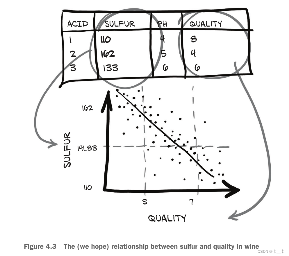
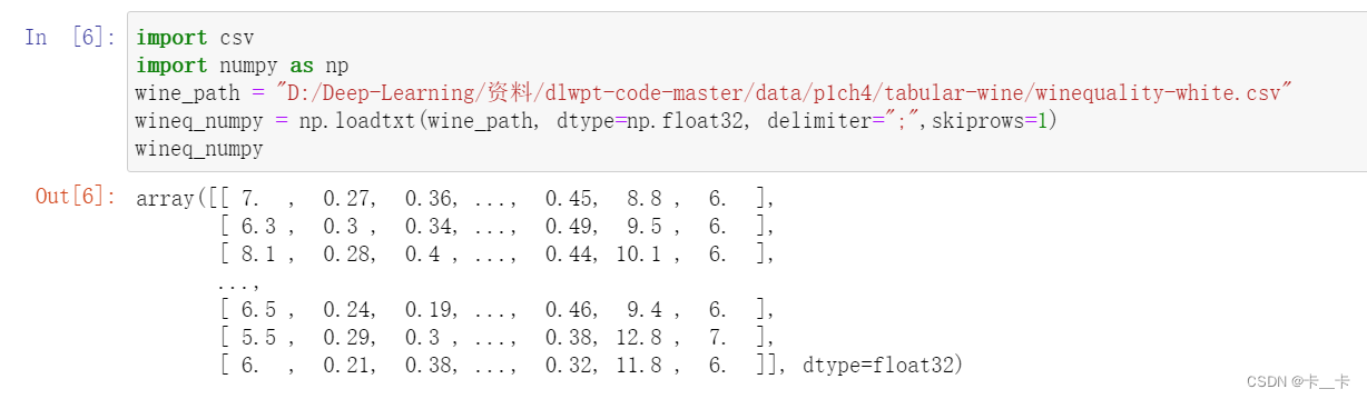
Let’s load our file and turn the resulting NumPy array into a PyTorch tensor.
import csv
import numpy as np
wine_path = "D:/Deep-Learning/资料/dlwpt-code-master/data/p1ch4/tabular-wine/winequality-white.csv"
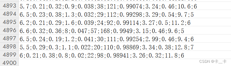
wineq_numpy = np.loadtxt(wine_path, dtype=np.float32, delimiter=";",skiprows=1)
# skiprows=1 表示跳过第一行的标题行
wineq_numpy
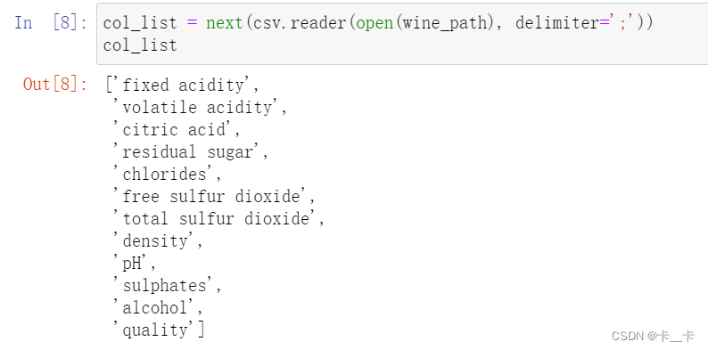
We can obtain column names (the first row of data) using this approach.
col_list = next(csv.reader(open(wine_path), delimiter=';'))
col_list
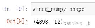
Let’s check that all the data has been read.
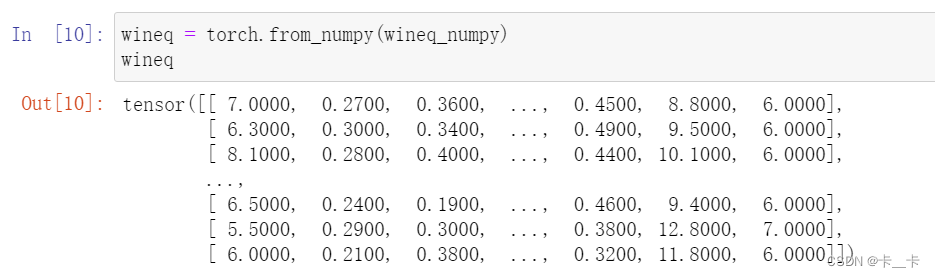
and proceed to convert the NumPy array to a PyTorch tensor:
wineq = torch.from_numpy(wineq_numpy)
wineq
wineq.shape, wineq.dtype
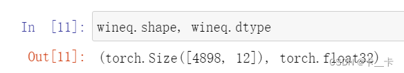
At this point, we have a floating-point torch.Tensor containing all the columns, including the last, which refers to the quality score.
Continuous, ordinal, and categorical values
continuous values: Stating that package A is 2 kilograms heavier than package B, or that package B came from 100 miles farther away than A has a fixed meaning. If you’re counting or measuring something with units, it’s probably a continuous value.
ordinal values: A good examplenof this is ordering a small, medium, or large drink, with small mapped to the value 1, medium 2, and large 3. The large drink is bigger than the medium, in the same way that 3 is bigger than 2, but it doesn’t tell us anything about how much bigger.
categorical values: Assigning water to 1, coffee to 2, soda to 3, and milk to 4 is a good example.
在处理一个包含scores(即quality)的问题时,可以将评分视为连续变量并进行回归任务,或将其视为标签并尝试从化学分析中猜测标签的分类任务。在这两种方法中,通常会从输入数据的张量中移除scores(下文data),并将其保存在一个单独的张量中(下文target),这样我们可以将score作为真实值使用,而不将其作为模型的输入。
将scores作为分类任务中的标签,而输入数据是基于化学分析的其他特征。这样的任务旨在根据给定的化学分析特征,通过模型预测和分类的方式来推断scores的标签或类别。通过这种方式,我们可以使用模型从输入数据中学习化学特征与评分之间的关联,并进行分类预测。
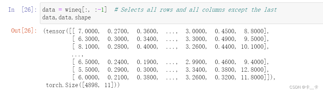
data = wineq[:, :-1]  # Selects all rows and all columns except the last
data,data.shape
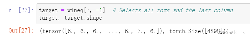
target = wineq[:, -1]  # Selects all rows and the last column
target, target.shape
标签张量(Label tensor)是一个包含离散标签值的张量。在分类任务中,我们通常将目标值(target)转换为标签张量,其中每个样本的目标值表示为一个整数,代表样本所属的类别或标签。标签张量的形状通常与输入数据的形状相对应,每个样本都有一个对应的标签值。
例如,如果我们有一个包含10个样本的数据集(可以将其看成表格的第一列),每个样本有3个特征(可以将其看成表格的第一行),而目标是将样本分为3个类别(标签为0、1和2),那么标签张量的形状将是(10,),其中每个元素表示一个样本的类别标签。(简单说,每一列就是一个标签张量)
标签张量在训练和评估模型时起着重要的作用。它用于计算损失函数,评估模型的性能,并与模型的预测进行比较,以确定预测是否正确。
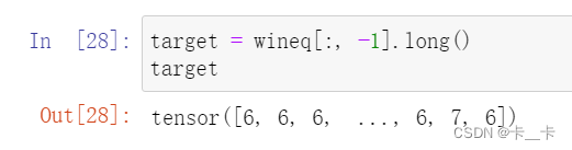
如果我们想把target转换成标签张量,一种方法是简单地将标签视为scores的整数向量:
target = wineq[:, -1].long()
target
另一种方法是构建分数的one-hot encoding
也就是说,在由10个元素组成的向量中对10个scores进行编码,所有元素都被设置为0(除了1),每个scores的索引都不同。这样,1的score可以映射到向量(1,0,0,0,0,0,0,0,0,0,0,0,0),5的score可以映射到(0,0,0,0,1,0,0,0,0,0),以此类推。
这两种方法有明显的区别。将葡萄酒质量scores保存在scores的整数向量中会对scores进行排序(例如1低于4)。它还能推导出分数之间的某种距离(1到3的距离=2到4的距离)。如果分数是纯粹离散的,就像葡萄品种,one-hot encoding将是一个更好的匹配,因为没有隐含的顺序或距离。
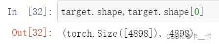
使用target.shape[0]即可表示样本数量
10表示类别总数
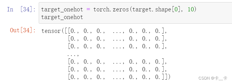
现在我们创建了一个全零张量target_onehot
target_onehot = torch.zeros(target.shape[0], 10)
我们可以使用scatter_ 方法实现one-hot encoding
名称以下划线结尾,表明该方法将不返回一个新的张量,而是在适当的地方修改张量
第一个参数1表示在维度1(列维度)上进行散布操作
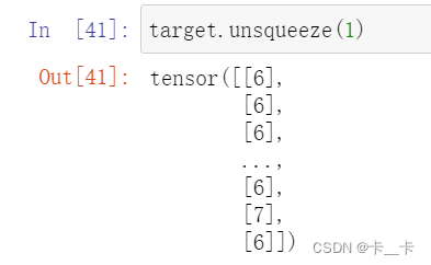
unsqueeze使target从[4898]变为[4898, 1],扩展后的张量就可以作为索引张量,用于指定在维度1上进行散布操作的位置
1.0表示按照目标标签的索引位置进行散布操作,即每个样本的目标标签对应的位置会被设置为1.0,而其他位置仍保持为0.0
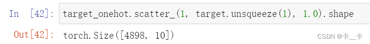
target_onehot.scatter_(1, target.unsqueeze(1), 1.0)
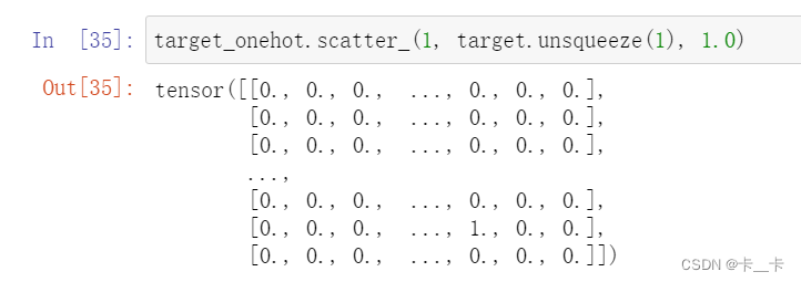
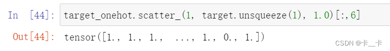
可以看到,第一行的第6个位置(从0起)被置为1(表示6)
倒数第二行的地7个位置(从0起)被置为1(表示7)
下面进行标准化
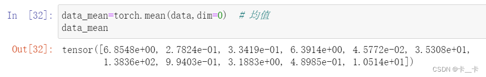
首先求各列的均值和标准差
data_mean=torch.mean(data,dim=0)  # 均值
data_mean
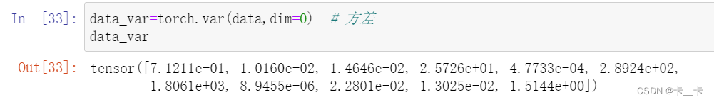
data_var=torch.var(data,dim=0)  # 方差
data_var
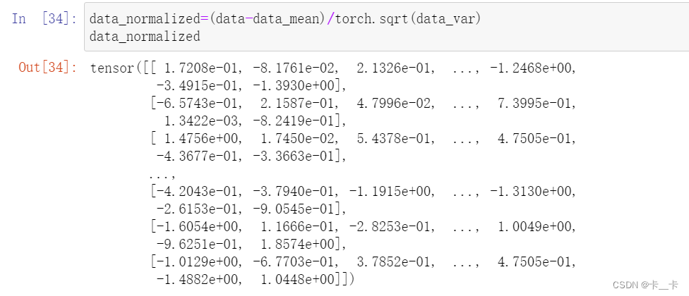
我们可以通过减去均值并除以标准差来标准化数据
data_normalized=(data-data_mean)/torch.sqrt(data_var)
data_normalized
我们来看看这些数据,是否有一种简单的方法可以一眼就分辨出葡萄酒的好坏。
First, we’re going to determine which rows in target correspond to a score less than or equal to 3:
bad_indexed=target<=3
bad_indexed
print(bad_indexed.shape)
print(bad_indexed.dtype)
print(bad_indexed.sum())
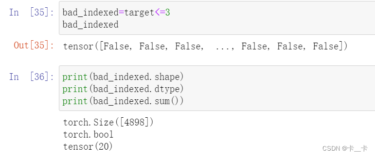
Note that only 20 of the bad_indexes entries are set to True.
For example,
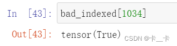
The bad_indexes tensor has the same shape as target, with values of False or True depending on the outcome of the comparison between our threshold and each element in the original target tensor:
bad_data=data[bad_indexed]
bad_data
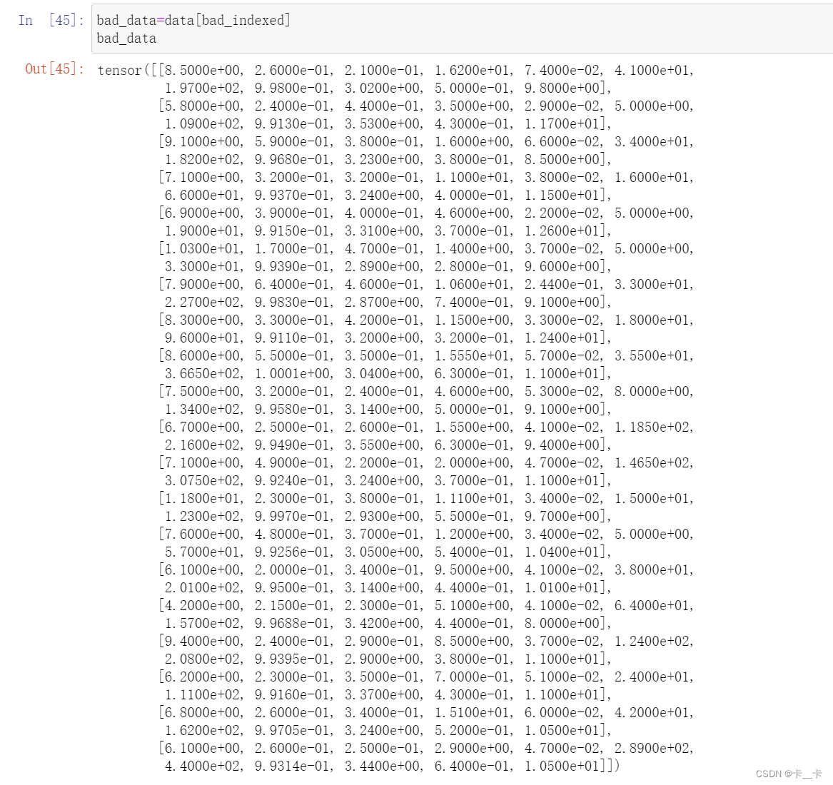
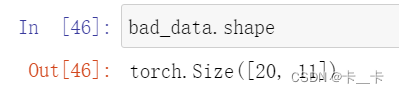
Note that the new bad_data tensor has 20 rows, the same as the number of rows with True in the bad_indexes tensor. It retains all 11 columns.
Now we can start to get information about wines grouped into good, middling, and bad categories. Let’s take the .mean() of each column:
bad_data=data[target<=3]
mid_data=data[(target>3)&(target<7)]
good_data=data[target>=7]
bad_mean=torch.mean(bad_data,dim=0)
mid_mean=torch.mean(mid_data,dim=0)
good_mean=torch.mean(good_data,dim=0)
zip函数将col_list、bad_mean、mid_mean和good_mean按索引依次配对,生成一个迭代器,每次迭代输出一个四元组。enumerate函数用于遍历这个迭代器,并返回每个元素及其对应的索引。i是索引,args是一个四元组,分别对应每个列的名称和其对应的坏、中等、好类别的平均值。在遍历过程中,可以使用i和args来处理每一列的数据和平均值。
format方法用于格式化输出字符串。前面输出5个,分别是i和args四元组,使用大括号格式化
‘{:2}’ :使用两个字符的宽度对齐,并且右对齐
‘{:20}’ :使用二十个字符的宽度对齐,并且左对齐。
‘{:6.2f}’ :使用六个字符的宽度对齐,其中两位小数,并且右对齐。
*args用于将四元组中的元素解包作为参数传递给format方法,这样可以按顺序填充格式化字符串中的占位符。通过这种方式,代码将索引、列名和平均值按指定格式输出为表格形式。
for i,args in enumerate(zip(col_list,bad_mean,mid_mean,good_mean)):
    print('{:2} {:20} {:6.2f} {:6.2f} {:6.2f}'.format(i,*args))
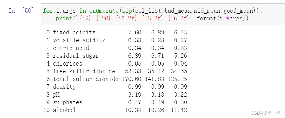
It looks like we’re on to something here: at first glance, the bad wines seem to have higher total sulfur dioxide, among other differences. We could use a threshold on total sulfur dioxide as a crude criterion for discriminating good wines from bad ones.
torch.lt(x, y) 比较 x 和 y 的每个元素,并返回一个布尔张量。x<y true,否则false
import torchx = torch.tensor([1, 2, 3, 4, 5])
y = torch.tensor([3, 3, 3, 3, 3])
result = torch.lt(x, y)
print(result) # Output: tensor([ True, True, False, False, False])`
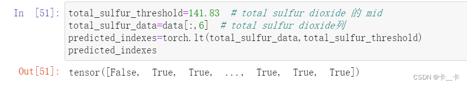
total_sulfur_threshold=141.83  # total sulfur dioxide 的 mid
total_sulfur_data=data[:,6]  # total sulfur dioxide列
predicted_indexes=torch.lt(total_sulfur_data,total_sulfur_threshold)
predicted_indexes
predicted_indexes.shape,predicted_indexes.dtype,predicted_indexes.sum()
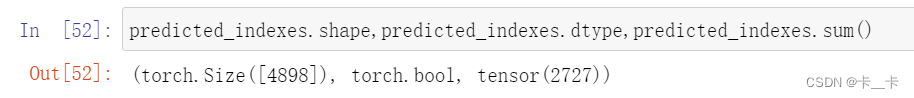
This means our threshold implies that just over half of all the wines are going to be high quality.
(total sulfur dioxide越小越好,有2727个小于threshold,即我们预测有2727瓶好酒)
Next, we’ll need to get the indexes of the actually good wines:
actual_indexes=target>5
actual_indexes.sum()
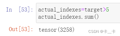
Since there are about 500 more actually good wines than our threshold predicted, we already have hard evidence that it’s not perfect.(之前拿>=7定义好酒,现在又改成5了,emmmm)
Now we need to see how well our predictions line up with the actual rankings. We will perform a logical “and” between our prediction indexes and the actual good indexes (remember that each is just an array of zeros and ones) and use that intersection of wines-in-agreement to determine how well we did:
当我们从一个张量中提取单个元素时,得到的是一个张量,而不是一个标量。这时,如果我们希望得到这个张量的数值值(即标量),可以使用.item() 方法。
x = torch.tensor(3.5)
value = x.item()
print(value) # 输出 3.5
n_matches = torch.sum(actual_indexes & predicted_indexes).item()
n_predicted = torch.sum(predicted_indexes).item()
n_actual = torch.sum(actual_indexes).item()
n_matches, n_matches / n_predicted, n_matches / n_actual
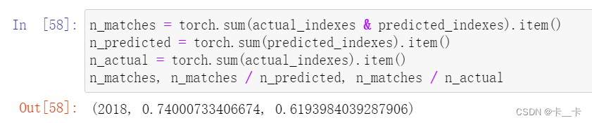
We got around 2,000 wines right! Since we predicted 2,700 wines, this gives us a 74% chance that if we predict a wine to be high quality, it actually is. Unfortunately, there are 3,200 good wines, and we only identified 61% of them. Well, we got what we signed up for; that’s barely better than random!
Of course, this is all very naive: we know for sure that multiple variables contribute to wine quality, and the relationships between the values of these variables and the outcome (which could be the actual score, rather than a binarized version of it) is likely more complicated than a simple threshold on a single value.