机器学习各个算法---1.线性回归

1.最原始的linear regression

标准回归函数和文本数据导入函数

from numpy import *

def loadDataSet(fileName):      #general function to parse tab -delimited floats
    numFeat = len(open(fileName).readline().split('\t')) - 1 #get number of fields '\t'是tab,每一行的特征个数
    dataMat = []; labelMat = []   #数据矩阵，标签矩阵
    fr = open(fileName)
    for line in fr.readlines():  #fr.readlines()表示读取每一行
        lineArr =[]   #该行的列表,注意这里保存的可是数字了
        curLine = line.strip().split('\t')  #strip()去掉前后的空格,split()把一个字符串分割成字符串数组
        for i in range(numFeat):   #数字序列，内置函数range() range(10) [0, 1, 2, 3, 4, 5, 6, 7, 8, 9]
            lineArr.append(float(curLine[i]))   #
        dataMat.append(lineArr)
        labelMat.append(float(curLine[-1]))  #-1表示倒数第一个
    return dataMat,labelMat    #返回数据矩阵和标签矩阵(目标值矩阵)

def standRegres(xArr,yArr):     #用来计算最佳拟合直线
    xMat = mat(xArr); yMat = mat(yArr).T   #搞成矩阵形式   matrix.T transpose：返回矩阵的转置矩阵
    xTx = xMat.T*xMat
    if linalg.det(xTx) == 0.0:     # numpy.linalg模块包含线性代数的函数,计算行列式值是否为0
        print "This matrix is singular, cannot do inverse"   #奇异矩阵
        return
    ws = xTx.I * (xMat.T*yMat)   #matrix.I inverse：返回矩阵的逆矩阵,就这一步就求出来了，该算法叫做普通最小二乘法(ordinary least squares)
    return ws

测试

import regression
import matplotlib.pyplot as plt
from numpy import *
xArr, yArr = regression.loadDataSet('ex0.txt')
# print xArr[0:2] #取不到2
# print yArr
#接下来来看拟合的效果
ws = regression.standRegres(xArr, yArr)
# print ws    #变量ws存放的就是回归系数
xMat = mat(xArr)
yMat = mat(yArr)
yHat = xMat*ws #计算预测值
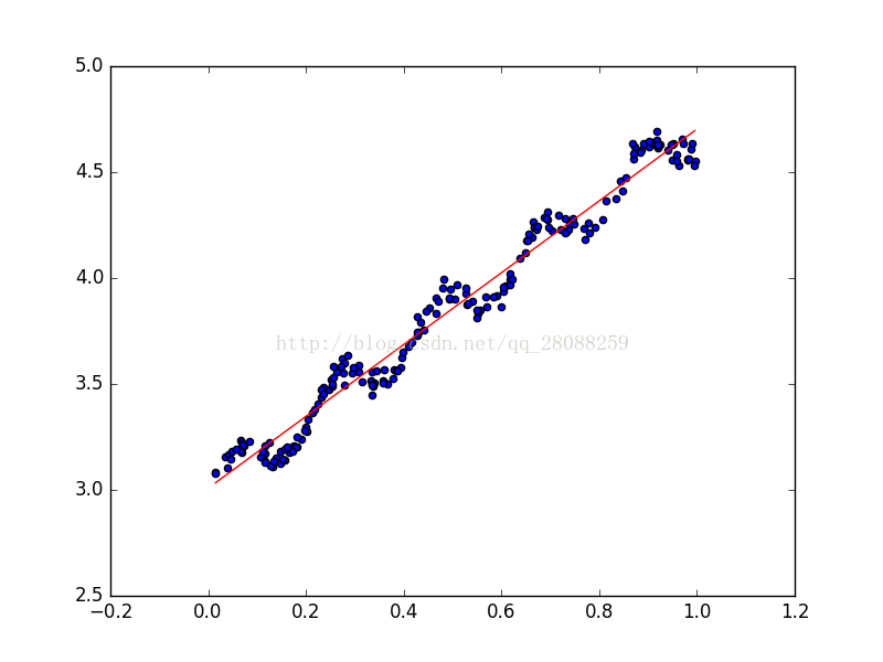
#接下来绘制数据集散点图和最佳拟合直线图
fig = plt.figure()
ax = fig.add_subplot(111)
ax.scatter(xMat[:,1].flatten().A[0],yMat.T[:,0].flatten().A[0]) 
# flatten()方法能将matrix的元素变成一维的，
# .A能使matrix变成array  


xCopy = xMat.copy()
# print xCopy
xCopy.sort(0)   #按照升序排序,主要是根据第二个元素
# print xCopy
yHat = xCopy *ws
ax.plot(xCopy[:,1],yHat,'red')
plt.show()

结果：

2. locally weighted linear regression

必要函数

#以下函数，对于x空间中的任意一个testPoint,输出其对应的预测值yHat
def lwlr(testPoint,xArr,yArr,k=1.0):   # 参数k控制衰减速度   1.0为默认值; testPoint为输入，函数返回根据局部加权线性回归得出的预测值
    xMat = mat(xArr); yMat = mat(yArr).T
    m = shape(xMat)[0]     #[0]指示的是行数，也就是样本点个数
    weights = mat(eye((m)))   #eye(m)主对角元素为1----对应于（m,m），其余为0 
    for j in range(m):                      #next 2 lines create weights matrix
        diffMat = testPoint - xMat[j,:]     
        weights[j,j] = exp(diffMat*diffMat.T/(-2.0*k**2))
    xTx = xMat.T * (weights * xMat)
    if linalg.det(xTx) == 0.0:
        print "This matrix is singular, cannot do inverse"
        return
    ws = xTx.I * (xMat.T * (weights * yMat))
    return testPoint * ws

def lwlrTest(testArr,xArr,yArr,k=1.0):  #loops over all the data points and applies lwlr to each one， k的默认值为1
    m = shape(testArr)[0]
    yHat = zeros(m)     #元素全为0的向量
    for i in range(m):
        yHat[i] = lwlr(testArr[i],xArr,yArr,k)
    return yHat

def lwlrTestPlot(xArr,yArr,k=1.0):  #same thing as lwlrTest except it sorts X first
    yHat = zeros(shape(yArr))       #easier for plotting
    xCopy = mat(xArr)
    xCopy.sort(0)
    for i in range(shape(xArr)[0]):
        yHat[i] = lwlr(xCopy[i],xArr,yArr,k)
    return yHat,xCopy

测试

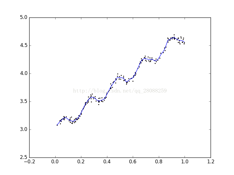
import regression
import matplotlib.pyplot as plt
from numpy import *

xArr, yArr = regression.loadDataSet('ex0.txt')
# print yArr[0]
# print regression.lwlr(xArr[0],xArr,yArr,0.001)
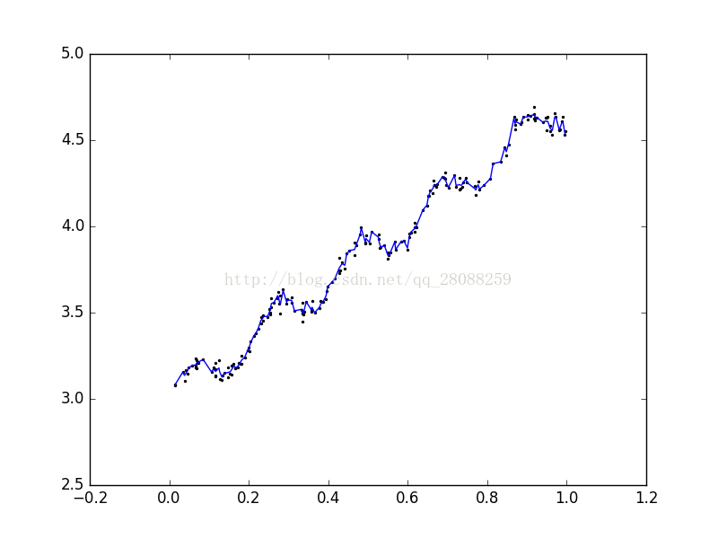
yHat, xSort = regression.lwlrTestPlot(xArr,yArr,1)    #此处的这个k值得选取会直接影响到拟合的效果
# print xSort

fig = plt.figure()
ax = fig.add_subplot(111)
ax.plot(xSort[:,1],yHat)
xMat = mat(xArr)
yMat = mat(yArr)
ax.scatter(xMat[:,1].flatten().A[0],yMat.T[:,0].flatten().A[0], s=2, c='red')
plt.show() 

k=1   欠拟合

k=0.01

k=0.003 过拟合

3. 预测鲍鱼的年龄

#预测鲍鱼年龄
import regression
from numpy import *

abX, abY = regression.loadDataSet('abalone.txt')
yHat01=regression.lwlrTest(abX[0:99],abX[0:99],abY[0:99],0.1)   #过拟合
yHat1=regression.lwlrTest(abX[0:99],abX[0:99],abY[0:99],1)
yHat10=regression.lwlrTest(abX[0:99],abX[0:99],abY[0:99],10)
print regression.rssError(abY[0:99], yHat01.T)
print regression.rssError(abY[0:99], yHat1.T)
print regression.rssError(abY[0:99], yHat10.T)

yHat01New=regression.lwlrTest(abX[100:199],abX[0:99],abY[0:99],0.1)   #过拟合
yHat1New=regression.lwlrTest(abX[100:199],abX[0:99],abY[0:99],1)
yHat10New=regression.lwlrTest(abX[100:199],abX[0:99],abY[0:99],10)
print regression.rssError(abY[100:199], yHat01New.T)
print regression.rssError(abY[100:199], yHat1New.T)
print regression.rssError(abY[100:199], yHat10New.T)

#接下里看看普通的线性回归
ws = regression.standRegres(abX[0:99], abY[0:99])
yHat =mat(abX[100:199])*ws
print regression.rssError(abY[100:199],yHat.T.A)

结果：

56.8843765879
429.89056187
549.118170883

58720.7256135
573.526144189
517.571190538

518.636315325

4. 缩减系数来“理解”数据

4.1 岭回归

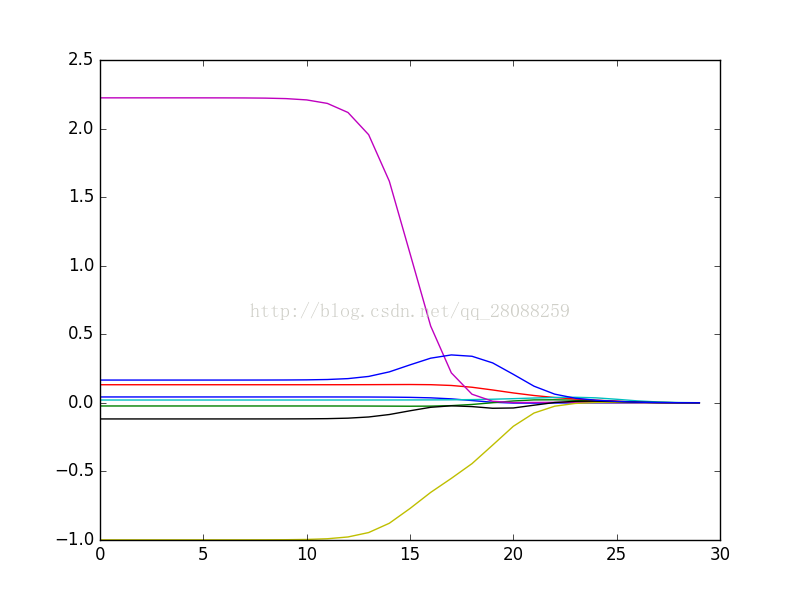
#岭回归---在鲍鱼数据集上的效果
import regression
from numpy import *
import matplotlib.pyplot as plt

abX, abY = regression.loadDataSet('abalone.txt')
ridgeWeights = regression.ridgeTest(abX, abY)
print ridgeWeights
fig = plt.figure()
ax = fig.add_subplot(111)
ax.plot(ridgeWeights)
plt.show()

4.2 前向逐步回归

def regularize(xMat):#regularize by columns
    inMat = xMat.copy()
    inMeans = mean(inMat,0)   #calc mean then subtract it off
    inVar = var(inMat,0)      #calc variance of Xi then divide by it
    inMat = (inMat - inMeans)/inVar
    return inMat

def stageWise(xArr,yArr,eps=0.01,numIt=100):    #前向逐步线性回归
    xMat = mat(xArr); yMat=mat(yArr).T
    yMean = mean(yMat,0)
    yMat = yMat - yMean     #can also regularize ys but will get smaller coef
    xMat = regularize(xMat)
    m,n=shape(xMat)
    returnMat = zeros((numIt,n)) #testing code remove
    ws = zeros((n,1)); wsTest = ws.copy(); wsMax = ws.copy()
    for i in range(numIt):   #numIt表示迭代次数
        print ws.T
        lowestError = inf;   #inf表示无穷
        for j in range(n):
            for sign in [-1,1]:   #分别显示增加和减少该特征系数对结果的影响
                wsTest = ws.copy()
                wsTest[j] += eps*sign
                yTest = xMat*wsTest
                rssE = rssError(yMat.A,yTest.A)
                if rssE < lowestError:
                    lowestError = rssE
                    wsMax = wsTest
        ws = wsMax.copy()
        returnMat[i,:]=ws.T
    return returnMat

测试

#测试前向逐步线性回归的效果
import regression
from numpy import *
import matplotlib.pyplot as plt

xArr, yArr = regression.loadDataSet('abalone.txt')
print regression.stageWise(xArr,yArr,0.001,5000)

#将其结果与最小二乘法进行比较
xMat = mat(xArr)
yMat = mat(yArr).T
xMat = regression.regularize(xMat)
yM = mean(yMat,0)
yMat = yMat - yM
weights=regression.standRegres(xMat, yMat.T)
print weights.T