Pytorch Tutorial【Chapter 3. Simple Neural Network】

文章目录

Pytorch Tutorial【Chapter 3. Simple Neural Network】

Chapter 3. Simple Neural Network

3.1 Train Neural Network Procedure训练神经网络流程

一个典型的神经网络训练过程包括以下几点：

定义一个包含可训练参数的神经网络
迭代整个输入
通过神经网络处理输入
计算损失(loss)
反向传播梯度到神经网络的参数
更新网络的参数，典型的用一个简单的更新方法：weight = weight - learning_rate *gradient

3.2 Build Neural Network Procedure 搭建神经网络

定义一个类并继承torch.nn.Moulde
使用类torch.nn中的组件和torch.nn.functional中的组件来搭建网络结构
改写该类的forward方法，在此方法中，进一步完善网络结构（如激活函数，池化层等），并且获得返回值的输出

先简要介绍一下需要使用到的torch.nn组件

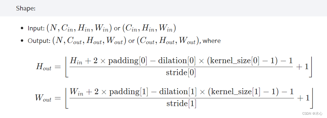
torch.nn.Conv2d(in_channels, out_channels, kernel_size)进行卷积操作，输入是 $N, C_{in},H,W)$ ，输出是 $N,C_{out},H,W)$ （详见Conv2d），卷积对图片尺寸的影响如下

torch.nn.Linear(in_features, out_features) 进行放射变换操作（affine mapping），即 $y=xA^T+b$ ，（详见Linear）
torch.nn.Flatten(start_dim=1, end_dim=- 1)，将连续的范围展平为张量（详见Flatten）

再介绍一下需要使用到的torch.nn.functional组件

扫描二维码关注公众号，回复： 16877112 查看本文章

torch.nn.functional.relu()，对输入使用Relu激活函数，具体操作是对每个元素都进行 $\text{ReLU}(x)=\max(0,x)$ 的计算，（详见ReLu）
torch.nn.functional.softmax()，对输入使用Softmax激活函数，具体操作是对每个元素都进行 $\text{Softmax}(x_i)=\frac{\exp(x_i)}{\sum_{j}\exp(x_j)}$ （详见Softmax）
torch.nn.functional.max_pool2d(input, kernel_size, stride) , 进行最大池化操作，输入是 $KaTeX parse error: Expected 'EOF', got '_' at position 28: …atch}, \text{in_̲channels}, iH,i…$ ，详见Max_Pool2D）

例如下述代码，我们要搭建一个下图的神经网络结构

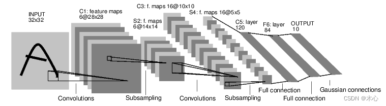
输入是 $[\text{batch},\text{channels},\text{height},\text{weight}]$ 的图片，分别代表批量大小、通道数、图像的高度、图像的宽度。在我们取批量大小为 $1$ ，然后这个例子变成 $[1, 1, 32, 32]$ ，张量的变化过程如下所示
$KaTeX parse error: Expected 'EOF', got '_' at position 74: …arrow{\text{max_̲pool}}[1,6,14,1…$

import torch
import torch.nn as nn
import torch.nn.functional as F

class Net(nn.Module):
    def __init__(self):
        super(Net,self).__init__()
        # 1 is input_channel 6 is output_channel
        self.conv1 = nn.Conv2d(1, 6, 5)
        self.conv2 = nn.Conv2d(6, 16, 5)
        # affine function y = Wx + b
        self.fc1 = nn.Linear(16 * 5 * 5, 120)
        self.fc2 = nn.Linear(120, 84)
        self.fc3 = nn.Linear(84, 10)
    
    def forward(self,x):
        # Max pooling over a (2,2) window
        x = F.max_pool2d(F.relu(self.conv1(x)), (2,2))
        # If the size is a square you can only specify a single number
        x = F.max_pool2d(F.relu(self.conv2(x)), (2,2))
        # flat the feature as a vector
        x = x.view(-1, self.num_flat_features(x))
        x = F.relu(self.fc1(x))
        x = F.relu(self.fc2(x))
        x = F.softmax(self.fc3(x), dim=1)
        return x


    def num_flat_features(self,x):
        size = x.size()[1:] # all dimensions except the batch dimension
        num_feature = 1
        for s in size:
            num_feature *= s
        return num_feature

net = Net()
print(net)

或

class Net(nn.Module):
    def __init__(self):
        super(Net,self).__init__()
        # 1 is input_channel 6 is output_channel
        self.conv1 = nn.Conv2d(1, 6, 5)
        self.conv2 = nn.Conv2d(6, 16, 5)
        # affine function y = Wx + b
        self.flat = nn.Flatten(1,-1)    # flat the feature
        self.fc1 = nn.Linear(16 * 5 * 5, 120)
        self.fc2 = nn.Linear(120, 84)
        self.fc3 = nn.Linear(84, 10)
    
    def forward(self,x):
        # Max pooling over a (2,2) window
        x = F.max_pool2d(F.relu(self.conv1(x)), (2,2))
        # If the size is a square you can only specify a single number
        x = F.max_pool2d(F.relu(self.conv2(x)), (2,2))
        # flat the feature as a vector
        x = self.flat(x)
        x = F.relu(self.fc1(x))
        x = F.relu(self.fc2(x))
        x = F.softmax(self.fc3(x), dim=1)
        return x


net = Net()
print(net)

结果如下，可以查看网络结构

Net(
  (conv1): Conv2d(1, 6, kernel_size=(5, 5), stride=(1, 1))
  (conv2): Conv2d(6, 16, kernel_size=(5, 5), stride=(1, 1))
  (fc1): Linear(in_features=400, out_features=120, bias=True)
  (fc2): Linear(in_features=120, out_features=84, bias=True)
  (fc3): Linear(in_features=84, out_features=10, bias=True)
)

一个模型可训练的参数可以通过调用 net.parameters() 返回，

params = list(net.parameters())
print(len(params))
print(params[0].size())  # conv1's .weight

结果如下

10
torch.Size([6, 1, 5, 5])

然后我们可以自定义一些输入，来获得网络的输出

input = torch.randn(3, 1, 32, 32)
out = net(input)
print(out.data)
sum = 0
for i in out.data[0]:
    sum += i.item()
print(sum)

输出如下

tensor([[0.0996, 0.1000, 0.0907, 0.0946, 0.0930, 0.1067, 0.1044, 0.1119, 0.1073,
         0.0918],
        [0.0975, 0.1005, 0.0913, 0.0935, 0.0939, 0.1070, 0.1045, 0.1121, 0.1065,
         0.0933],
        [0.0968, 0.1009, 0.0896, 0.0978, 0.0903, 0.1107, 0.1055, 0.1130, 0.1043,
         0.0913]])
0.9999999925494194

torch.nn.Module.zero_grad()把所有参数梯度缓存器置零，

net.zero_grad() #把所有参数梯度缓存器置零，用随机的梯度来反向传播
out.backward(torch.randn_like(out))
net.conv1.bias.grad  #查看Conv卷积层的偏置和权重一些参数的梯度
net.conv1.weight.grad

结果如下

tensor([-0.0064,  0.0136, -0.0046,  0.0008, -0.0044,  0.0021])
...

3.3 Use Loss Function to Backward 利用损失函数进行反向传播

现在我们已经完成了

定义一个神经网络
处理输入以及调用反向传播

还剩下：

计算损失值
更新网络中的权重

损失函数

一个损失函数需要一对输入：模型输出和目标，然后计算一个值来评估输出距离目标有多远。

有一些不同的损失函数在 nn 包（详细请查看loss-functions）。一个简单的损失函数就是 nn.MSELoss ，这计算了均方误差

input = torch.randn(3, 1, 32, 32)
target = torch.randn(3, 10)
predict = net(input)
criterion = nn.MSELoss()
loss = criterion(predict, target)

print(loss)
print(loss.grad_fn.next_functions[0][0])

我们计算了MSE损失函数，并且能够跟踪其计算图

input -> conv2d -> relu -> maxpool2d -> conv2d -> relu -> maxpool2d
      -> view -> linear -> relu -> linear -> relu -> linear -> sfotmax
      -> MSELoss
      -> loss

当我们使用loss.backward()时，整个计算图都会进行微分，为了实现反向传播损失，我们所有需要做的事情仅仅是使用 loss.backward()。你需要清空现存的梯度，要不然现在计算的梯度都将会和历史保存的梯度累计到一起。

net.zero_grad()     # zeroes the gradient buffers of all parameters

print('conv1.bias.grad before backward')
print(net.conv1.bias.grad)

loss.backward()

print('conv1.bias.grad after backward')
print(net.conv1.bias.grad)

结果如下

conv1.bias.grad before backward
None
conv1.bias.grad after backward
tensor([-3.4418e-04, -1.0766e-04,  1.0913e-04, -5.5018e-05,  1.7342e-04,
        -5.3316e-04])

3.4 Update Parameter of NN 更新神经网络参数

3.4.1 Update Manually手动更新参数

我们可以手动实现随机梯度下降（stochastic gradient descent）来更新参数（详细请参考Chapter 6. Stochastic Approximation）

$\textcolor{red}{w_{k+1} = w_k - a_k \nabla_{w_k} f(w_k,x_k)}$

learning_rate = 0.01
for f in net.parameters():
    f.data.sub_(f.grad.data * learning_rate)    #sub_() is in-place minus

3.4.2 Update Automatically自动更新参数

尽管如此，如果你是用神经网络，你想使用不同的更新规则，类似于 SGD, Nesterov-SGD, Adam, RMSProp, 等。为了让这可行，我们建立了一个小包：torch.optim 实现了所有的方法。我们可以使用optim.step()来替代上述手动实现的代码，使用它非常的简单。

import torch.optim as optim

# create your optimizer
optimizer = optim.SGD(net.parameters(), lr=0.01)

# in your training loop:
optimizer.zero_grad()   # zero the gradient buffers
output = net(input)
loss = criterion(output, target)	
loss.backward()		# 计算梯度
optimizer.step()    # Does the update

Reference

参考教程1
参考教程2