简单的线性回归
我们先写一个简单的线性回归练练手
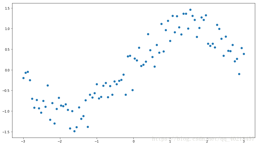
实际的数据大家可以通过pandas等package读入,也可以使用自带的Boston House Price数据集,这里为了简单,我们自己手造一点数据集。
In [1]:
%matplotlib inline# 在notebook里面显示图像
import numpy as np
import tensorflow as tf
import matplotlib.pyplot as plt
plt.rcParams["figure.figsize"] = (14,8)# 显示图像的最大范围

n_observations = 100
xs = np.linspace(-3, 3, n_observations)#linspace函数可以生成元素为50的等间隔数列。而前两个参数分别是数列的开头与结尾。如果写入第三个参数,可以制定数列的元素个数。
ys = np.sin(xs) + np.random.uniform(-0.5, 0.5, n_observations)#:从一个均匀分布[low,high)中随机采样,
plt.scatter(xs, ys)
plt.show()
In [2]:
X = tf.placeholder(tf.float32, name='X')
Y = tf.placeholder(tf.float32, name='Y')
In [3]:
W = tf.Variable(tf.random_normal([1]), name='weight')#tf.random_normal函数用于从服从指定正太分布的数值中取出指定个数的值。
b = tf.Variable(tf.random_normal([1]), name='bias')
In [4]:
Y_pred = tf.add(tf.multiply(X, W), b)#y=wx+b
In [5]:
loss = tf.square(Y - Y_pred, name='loss')
In [6]:
learning_rate = 0.01
optimizer = tf.train.GradientDescentOptimizer(learning_rate).minimize(loss)
In [7]:
n_samples = xs.shape[0]
with tf.Session() as sess:
	# 记得初始化所有变量
	sess.run(tf.global_variables_initializer())

	writer = tf.summary.FileWriter('./graphs/linear_reg', sess.graph)#写到日志这里的点代表python所在的路径

	# 训练模型
	for i in range(50):
		total_loss = 0
		for x, y in zip(xs, ys):#zip() 函数用于将可迭代的对象作为参数,将对象中对应的元素打包成一个个元组,然后返回由这些元组组成的列表。
			# 通过feed_dict字典把数据灌进去
			_, l = sess.run([optimizer, loss], feed_dict={X: x, Y:y}) #_,l分别得到optimizer,loss


			total_loss += l
		if i%5 ==0:
			print('Epoch {0}: {1}'.format(i, total_loss/n_samples))#取平均值total_loss/n_samples


	# 关闭writer
	writer.close()

	# 取出w和b的值
	W, b = sess.run([W, b])
In [8]:
print(W,b)
print("W:"+str(W[0]))
print("b:"+str(b[0]))
In [9]:
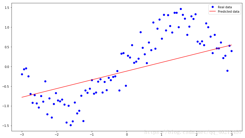
plt.plot(xs, ys, 'bo', label='Real data')
plt.plot(xs, xs * W + b, 'r', label='Predicted data')
plt.legend()
plt.show()
plt.plot(x,y,format_string,**kwargs)
x轴数据,y轴数据,format_string控制曲线的格式字串
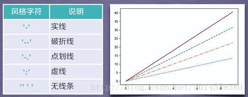
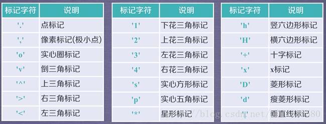
format_string 由颜色字符,风格字符,和标记字符
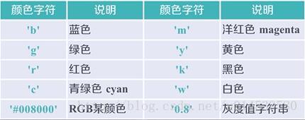
x轴数据,y轴数据,format_string控制曲线的格式字串
format_string 由颜色字符,风格字符,和标记字符
多项式回归
by @寒小阳
对于非线性的数据分布,用线性回归拟合程度一般,我们来试试多项式回归
实际的数据大家可以通过pandas等package读入,也可以使用自带的Boston House Price数据集,这里为了简单,我们自己手造一点数据集。
In [1]:
%matplotlib inline
import numpy as np
import tensorflow as tf
import matplotlib.pyplot as plt
plt.rcParams["figure.figsize"] = (14,8)

n_observations = 100
xs = np.linspace(-3, 3, n_observations)
ys = np.sin(xs) + np.random.uniform(-0.5, 0.5, n_observations)
plt.scatter(xs, ys)
plt.show()
In [2]:
X = tf.placeholder(tf.float32, name='X')
Y = tf.placeholder(tf.float32, name='Y')
In [3]:
#tf.random_normal(shape, mean=0.0, stddev=1.0, dtype=tf.float32, seed=None, name=None)
- shape: 输出张量的形状,必选
- mean: 正态分布的均值,默认为0
- stddev: 正态分布的标准差,默认为1.0
- dtype: 输出的类型,默认为tf.float32
- seed: 随机数种子,是一个整数,当设置之后,每次生成的随机数都一样
- name: 操作的名称
W = tf.Variable(tf.random_normal([1]), name='weight')

b = tf.Variable(tf.random_normal([1]), name='bias')
In [4]:
#y=wx+w2*x^2+w3*x^3
Y_pred = tf.add(tf.multiply(X, W), b)
#添加高次项
W_2 = tf.Variable(tf.random_normal([1]), name='weight_2')
Y_pred = tf.add(tf.multiply(tf.pow(X, 2), W_2), Y_pred)#tf.pow次方
W_3 = tf.Variable(tf.random_normal([1]), name='weight_3')
Y_pred = tf.add(tf.multiply(tf.pow(X, 3), W_3), Y_pred)
In [5]:
sample_num = xs.shape[0]
loss = tf.reduce_sum(tf.pow(Y_pred - Y, 2)) / sample_num
In [6]:
learning_rate = 0.01
optimizer = tf.train.GradientDescentOptimizer(learning_rate).minimize(loss)
In [7]:
n_samples = xs.shape[0]
with tf.Session() as sess:
	# 记得初始化所有变量
	sess.run(tf.global_variables_initializer())

	writer = tf.summary.FileWriter('./graphs/polynomial_reg', sess.graph)

	# 训练模型
	for i in range(1000):
		total_loss = 0
		for x, y in zip(xs, ys):
			# 通过feed_dic把数据灌进去
			_, l = sess.run([optimizer, loss], feed_dict={X: x, Y:y})
			total_loss += l
		if i%20 ==0:
			print('Epoch {0}: {1}'.format(i, total_loss/n_samples))

	# 关闭writer
	writer.close()
    # 取出w和b的值
	W, W_2, W_3, b = sess.run([W, W_2, W_3, b])
In [8]:
print("W:"+str(W[0]))#第0个元素
print("W_2:"+str(W_2[0]))
print("W_3:"+str(W_3[0]))
print("b:"+str(b[0]))
In [9]:
plt.plot(xs, ys, 'bo', label='Real data')
plt.plot(xs, xs*W + np.power(xs,2)*W_2 + np.power(xs,3)*W_3 + b, 'r', label='Predicted data')
plt.legend()
plt.show()
逻辑回归
by @寒小阳
解决分类问题里最普遍的baseline model就是逻辑回归,简单同时可解释性好,使得它大受欢迎,我们来用tensorflow完成这个模型的搭建。
In [1]:
import os
os.environ['TF_CPP_MIN_LOG_LEVEL']='2'

import numpy as np
import tensorflow as tf
from tensorflow.examples.tutorials.mnist import input_data
import time
In [2]:
#使用tensorflow自带的工具加载MNIST手写数字集合
mnist = input_data.read_data_sets('/data/mnist', one_hot=True)
In [3]:
#查看一下数据维度
mnist.train.images.shape
Out[3]:
In [4]:
#查看target维度
mnist.train.labels.shape
Out[4]:
In [5]:
batch_size = 128
X = tf.placeholder(tf.float32, [batch_size, 784], name='X_placeholder')#X = tf.placeholder(tf.float32, [None, 784], name='X_placeholder')
                                                                               可以只指定维度不指定个数
Y = tf.placeholder(tf.int32, [batch_size, 10], name='Y_placeholder')
In [6]:
w = tf.Variable(tf.random_normal(shape=[784, 10], stddev=0.01), name='weights')#x*w+b 矩阵要能运算所以【784,10】
b = tf.Variable(tf.zeros([1, 10]), name="bias")
In [7]:
logits = tf.matmul(X, w) + b
In [8]:
# 求交叉熵损失
entropy = tf.nn.softmax_cross_entropy_with_logits(logits=logits, labels=Y, name='loss')
# 求平均
loss = tf.reduce_mean(entropy)
In [9]:
learning_rate = 0.01
optimizer = tf.train.AdamOptimizer(learning_rate).minimize(loss)
In [10]:
#迭代总轮次
n_epochs = 30

with tf.Session() as sess:
	# 在Tensorboard里可以看到图的结构
	writer = tf.summary.FileWriter('./graphs/logistic_reg', sess.graph)

	start_time = time.time()
	sess.run(tf.global_variables_initializer())
	n_batches = int(mnist.train.num_examples/batch_size)
	for i in range(n_epochs): # 迭代这么多轮
		total_loss = 0

		for _ in range(n_batches):
			X_batch, Y_batch = mnist.train.next_batch(batch_size)
			_, loss_batch = sess.run([optimizer, loss], feed_dict={X: X_batch, Y:Y_batch})
			total_loss += loss_batch
		print('Average loss epoch {0}: {1}'.format(i, total_loss/n_batches))

	print('Total time: {0} seconds'.format(time.time() - start_time))

	print('Optimization Finished!')

	# 测试模型

	preds = tf.nn.softmax(logits)
	correct_preds = tf.equal(tf.argmax(preds, 1), tf.argmax(Y, 1))#tf.argmax(preds,1)预测的0-9的一个数,
tf.argmax(preds,1)实际0-9的一个数
accuracy = tf . reduce_sum ( tf . cast ( correct_preds , tf . float32 )) #准确率
tf.cast(x, dtype, name=None)
此函数是类型转换函数
参数
- x:输入
- dtype:转换目标类型
- name:名称
多层感知器
by @寒小阳
我们来搭建第一个神经网络完成分类问题,这里依旧用刚才的手写数字识别问题为例。
In [1]:
import numpy as np
import tensorflow as tf
from tensorflow.examples.tutorials.mnist import input_data
import time
In [2]:
#使用tensorflow自带的工具加载MNIST手写数字集合
mnist = input_data.read_data_sets('/data/mnist', one_hot=True)
In [3]:
#查看一下数据维度
mnist.train.images.shape
Out[3]:
In [4]:
#查看target维度
mnist.train.labels.shape
Out[4]:
In [5]:
X = tf.placeholder(tf.float32, [None, 784], name='X_placeholder')
Y = tf.placeholder(tf.int32, [None, 10], name='Y_placeholder')
In [6]:
# 网络参数
n_hidden_1 = 256 # 第1个隐层
n_hidden_2 = 256 # 第2个隐层
n_input = 784 # MNIST 数据输入(28*28*1=784)
n_classes = 10 # MNIST 总共10个手写数字类别

weights = {
    'h1': tf.Variable(tf.random_normal([n_input, n_hidden_1]), name='W1'),#字典
    'h2': tf.Variable(tf.random_normal([n_hidden_1, n_hidden_2]), name='W2'),
    'out': tf.Variable(tf.random_normal([n_hidden_2, n_classes]), name='W')
}
biases = {
    'b1': tf.Variable(tf.random_normal([n_hidden_1]), name='b1'),
    'b2': tf.Variable(tf.random_normal([n_hidden_2]), name='b2'),
    'out': tf.Variable(tf.random_normal([n_classes]), name='bias')
}
In [7]:
def multilayer_perceptron(x, weights, biases):
    # 第1个隐层,使用relu激活函数
    layer_1 = tf.add(tf.matmul(x, weights['h1']), biases['b1'], name='fc_1')#x*w1=b1
    layer_1 = tf.nn.relu(layer_1, name='relu_1')#
使用relu激活函数
# 第2个隐层,使用relu激活函数
layer_2
=
tf
.
add
(
tf
.
matmul
(
layer_1
,
weights
[
'h2'
]),
biases
[
'b2'
],
name
=
'fc_2'
)
layer_2
=
tf
.
nn
.
relu
(
layer_2
,
name
=
'relu_2'
)
# 输出层
out_layer
=
tf
.
add
(
tf
.
matmul
(
layer_2
,
weights
[
'out'
]),
biases
[
'out'
],
name
=
'fc_3'
)
return
out_layer
In [8]:
pred = multilayer_perceptron(X, weights, biases)
In [9]:
learning_rate = 0.001
loss_all = tf.nn.softmax_cross_entropy_with_logits(logits=pred, labels=Y, name='cross_entropy_loss')#交叉熵
loss = tf.reduce_mean(loss_all, name='avg_loss')
optimizer = tf.train.AdamOptimizer(learning_rate=learning_rate).minimize(loss)
In [10]:
init = tf.global_variables_initializer()
In [11]:
#训练总轮数
training_epochs = 15
#一批数据大小
batch_size = 128
#信息展示的频度
display_step = 1

with tf.Session() as sess:
    sess.run(init)
    writer = tf.summary.FileWriter('./graphs/MLP_DNN', sess.graph)

    # 训练
    for epoch in range(training_epochs):
        avg_loss = 0.
        total_batch = int(mnist.train.num_examples/batch_size)
        # 遍历所有的batches
        for i in range(total_batch):
            batch_x, batch_y = mnist.train.next_batch(batch_size)
            # 使用optimizer进行优化
            _, l = sess.run([optimizer, loss], feed_dict={X: batch_x, Y: batch_y})
            # 求平均的损失
            avg_loss += l / total_batch
        # 每一步都展示信息
        if epoch % display_step == 0:
            print("Epoch:", '%04d' % (epoch+1), "cost=", \
                "{:.9f}".format(avg_loss))
    print("Optimization Finished!")

    # 在测试集上评估
    correct_prediction = tf.equal(tf.argmax(pred, 1), tf.argmax(Y, 1))
    # 计算准确率
    accuracy = tf.reduce_mean(tf.cast(correct_prediction, "float"))
    print("Accuracy:", accuracy.eval({X: mnist.test.images, Y: mnist.test.labels}))
    writer.close()