目录
利用padas、numpy、matplotlib、seaborn库,对数据进行分析。
Iris数据集是非常著名的机器学习数据集之一,在统计学和机器学习领域被广泛应用。该数据集包含了150个样本,分别来自三种不同的鸢尾花(Iris)品种:山鸢尾(setosa)、变色鸢尾(versicolor)和维吉尼亚鸢尾(virginica)。
每个样本包含了4个特征:花萼长度(sepal length)、花萼宽度(sepal width)、花瓣长度(petal length)和花瓣宽度(petal width)。根据这些特征,我们可以将鸢尾花分为不同的种类。
Iris数据集常被用来进行分类和聚类的实验,以及各种机器学习算法的训练和测试。它是一个相对简单的数据集,但具有一定的挑战性,特别是对于不平衡数据和其他相关问题的处理。
该数据集可以从很多机器学习软件包中获取,如scikit-learn库。通过使用这个数据集,我们可以训练模型来预测鸢尾花的品种,或者进行聚类以发现潜在的模式。
numpy:Numpy库-CSDN博客
padas:Pandas库-CSDN博客
matplotlib:matplotlib-CSDN博客
seaborn:seaborn库图形进行数据分析(基于tips数据集)-CSDN博客
import pandas as pd
import numpy as np
import matplotlib.pyplot as plt
import seaborn as sns
df=sns.load_dataset('iris')
'''结果:
 	sepal_length 	sepal_width 	petal_length 	petal_width 	species
0 	    5.1 	        3.5 	        1.4 	         0.2 	    setosa
1 	    4.9 	        3.0 	        1.4 	         0.2 	    setosa
2 	    4.7 	        3.2 	        1.3 	         0.2 	    setosa
3 	    4.6 	        3.1 	        1.5 	         0.2 	    setosa
4 	    5.0 	        3.6 	        1.4 	         0.2 	    setosa
... 	... 	... 	... 	... 	...
145 	6.7 	        3.0 	        5.2 	         2.3 	    virginica
146 	6.3 	        2.5 	        5.0 	         1.9 	    virginica
147 	6.5 	        3.0 	        5.2 	         2.0 	    virginica
148 	6.2 	        3.4 	        5.4 	         2.3 	    virginica
149 	5.9 	        3.0 	        5.1 	         1.8 	    virginica

150 rows × 5 columns

'''

type(df)
#结果:pandas.core.frame.DataFrame
一、数据处理
df['species'].unique()#有几种(唯一的)
#结果:array(['setosa', 'versicolor', 'virginica'], dtype=object)

df['species']=='setosa'
'''结果:
0       True
1       True
2       True
3       True
4       True
       ...
145    False
146    False
147    False
148    False
149    False
Name: species, Length: 150, dtype: bool
'''

df.loc[df['species']=='setosa']
'''结果:
sepal_length 	sepal_width 	petal_length 	petal_width 	species
0 	5.1 	3.5 	1.4 	0.2 	setosa
1 	4.9 	3.0 	1.4 	0.2 	setosa
2 	4.7 	3.2 	1.3 	0.2 	setosa
3 	4.6 	3.1 	1.5 	0.2 	setosa
4 	5.0 	3.6 	1.4 	0.2 	setosa
5 	5.4 	3.9 	1.7 	0.4 	setosa
6 	4.6 	3.4 	1.4 	0.3 	setosa
7 	5.0 	3.4 	1.5 	0.2 	setosa
8 	4.4 	2.9 	1.4 	0.2 	setosa
9 	4.9 	3.1 	1.5 	0.1 	setosa
10 	5.4 	3.7 	1.5 	0.2 	setosa
11 	4.8 	3.4 	1.6 	0.2 	setosa
12 	4.8 	3.0 	1.4 	0.1 	setosa
13 	4.3 	3.0 	1.1 	0.1 	setosa
14 	5.8 	4.0 	1.2 	0.2 	setosa
15 	5.7 	4.4 	1.5 	0.4 	setosa
16 	5.4 	3.9 	1.3 	0.4 	setosa
17 	5.1 	3.5 	1.4 	0.3 	setosa
18 	5.7 	3.8 	1.7 	0.3 	setosa
19 	5.1 	3.8 	1.5 	0.3 	setosa
20 	5.4 	3.4 	1.7 	0.2 	setosa
21 	5.1 	3.7 	1.5 	0.4 	setosa
22 	4.6 	3.6 	1.0 	0.2 	setosa
23 	5.1 	3.3 	1.7 	0.5 	setosa
24 	4.8 	3.4 	1.9 	0.2 	setosa
25 	5.0 	3.0 	1.6 	0.2 	setosa
26 	5.0 	3.4 	1.6 	0.4 	setosa
27 	5.2 	3.5 	1.5 	0.2 	setosa
28 	5.2 	3.4 	1.4 	0.2 	setosa
29 	4.7 	3.2 	1.6 	0.2 	setosa
30 	4.8 	3.1 	1.6 	0.2 	setosa
31 	5.4 	3.4 	1.5 	0.4 	setosa
32 	5.2 	4.1 	1.5 	0.1 	setosa
33 	5.5 	4.2 	1.4 	0.2 	setosa
34 	4.9 	3.1 	1.5 	0.2 	setosa
35 	5.0 	3.2 	1.2 	0.2 	setosa
36 	5.5 	3.5 	1.3 	0.2 	setosa
37 	4.9 	3.6 	1.4 	0.1 	setosa
38 	4.4 	3.0 	1.3 	0.2 	setosa
39 	5.1 	3.4 	1.5 	0.2 	setosa
40 	5.0 	3.5 	1.3 	0.3 	setosa
41 	4.5 	2.3 	1.3 	0.3 	setosa
42 	4.4 	3.2 	1.3 	0.2 	setosa
43 	5.0 	3.5 	1.6 	0.6 	setosa
44 	5.1 	3.8 	1.9 	0.4 	setosa
45 	4.8 	3.0 	1.4 	0.3 	setosa
46 	5.1 	3.8 	1.6 	0.2 	setosa
47 	4.6 	3.2 	1.4 	0.2 	setosa
48 	5.3 	3.7 	1.5 	0.2 	setosa
49 	5.0 	3.3 	1.4 	0.2 	setosa
'''
df_setosa=df.loc[df['species']=='setosa']
df_virginica=df.loc[df['species']=='virginica']
df_versicolor=df.loc[df['species']=='versicolor']#生成子表
df_versicolor.count()
'''结果:
sepal_length 50
sepal_width 50
petal_length 50
petal_width 50
species 50
dtype: int64
'''
df_setosa
'''结果:
sepal_length sepal_width petal_length petal_width species
0 5.1 3.5 1.4 0.2 setosa
1 4.9 3.0 1.4 0.2 setosa
2 4.7 3.2 1.3 0.2 setosa
3 4.6 3.1 1.5 0.2 setosa
4 5.0 3.6 1.4 0.2 setosa
5 5.4 3.9 1.7 0.4 setosa
6 4.6 3.4 1.4 0.3 setosa
7 5.0 3.4 1.5 0.2 setosa
8 4.4 2.9 1.4 0.2 setosa
9 4.9 3.1 1.5 0.1 setosa
10 5.4 3.7 1.5 0.2 setosa
11 4.8 3.4 1.6 0.2 setosa
12 4.8 3.0 1.4 0.1 setosa
13 4.3 3.0 1.1 0.1 setosa
14 5.8 4.0 1.2 0.2 setosa
15 5.7 4.4 1.5 0.4 setosa
16 5.4 3.9 1.3 0.4 setosa
17 5.1 3.5 1.4 0.3 setosa
18 5.7 3.8 1.7 0.3 setosa
19 5.1 3.8 1.5 0.3 setosa
20 5.4 3.4 1.7 0.2 setosa
21 5.1 3.7 1.5 0.4 setosa
22 4.6 3.6 1.0 0.2 setosa
23 5.1 3.3 1.7 0.5 setosa
24 4.8 3.4 1.9 0.2 setosa
25 5.0 3.0 1.6 0.2 setosa
26 5.0 3.4 1.6 0.4 setosa
27 5.2 3.5 1.5 0.2 setosa
28 5.2 3.4 1.4 0.2 setosa
29 4.7 3.2 1.6 0.2 setosa
30 4.8 3.1 1.6 0.2 setosa
31 5.4 3.4 1.5 0.4 setosa
32 5.2 4.1 1.5 0.1 setosa
33 5.5 4.2 1.4 0.2 setosa
34 4.9 3.1 1.5 0.2 setosa
35 5.0 3.2 1.2 0.2 setosa
36 5.5 3.5 1.3 0.2 setosa
37 4.9 3.6 1.4 0.1 setosa
38 4.4 3.0 1.3 0.2 setosa
39 5.1 3.4 1.5 0.2 setosa
40 5.0 3.5 1.3 0.3 setosa
41 4.5 2.3 1.3 0.3 setosa
42 4.4 3.2 1.3 0.2 setosa
43 5.0 3.5 1.6 0.6 setosa
44 5.1 3.8 1.9 0.4 setosa
45 4.8 3.0 1.4 0.3 setosa
46 5.1 3.8 1.6 0.2 setosa
47 4.6 3.2 1.4 0.2 setosa
48 5.3 3.7 1.5 0.2 setosa
49 5.0 3.3 1.4 0.2 setosa
'''二、单变量分析
plt.plot(df_setosa['sepal_length'])
plt.plot(df_versicolor['sepal_length'])
plt.plot(df_virginica['sepal_length'])
plt.ylabel('sepal_length')
plt.show()
plt.plot(df_setosa['sepal_length'],marker="x")
plt.plot(df_versicolor['sepal_length'],marker="*")
plt.plot(df_virginica['sepal_length'],marker="o")
plt.ylabel('sepal_length')
plt.show() 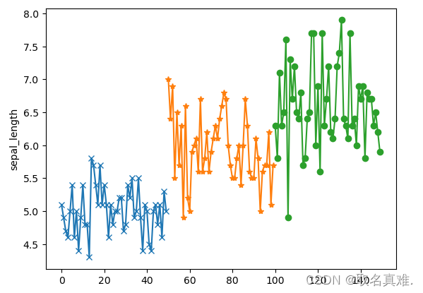
plt.plot(df_setosa['species'],df_setosa['sepal_length'],marker="o")
plt.plot(df_versicolor['species'],df_versicolor['sepal_length'],marker="o")
plt.plot(df_virginica['species'],df_virginica['sepal_length'],marker="o")
plt.ylabel('sepal_length')
plt.show() 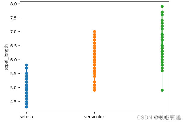
plt.plot(df_setosa['sepal_length'],np.zeros_like(df_setosa['sepal_length']),"o")
plt.plot(df_versicolor['sepal_length'],np.zeros_like(df_versicolor['sepal_length']),"x")
plt.plot(df_virginica['sepal_length'],np.zeros_like(df_virginica['sepal_length']),"*")#以0为轴
plt.ylabel('sepal_length')
plt.show() 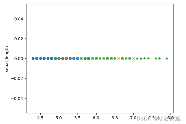
plt.plot(df_setosa['petal_length'],np.ones_like(df_setosa['sepal_length']),"o")
plt.plot(df_versicolor['petal_length'],np.ones_like(df_versicolor['sepal_length']),"x")
plt.plot(df_virginica['petal_length'],np.ones_like(df_virginica['sepal_length']),"*")#以一为轴
plt.ylabel('petal_length')
plt.show() 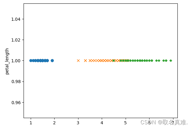
plt.hist(df["petal_length"])#柱状图 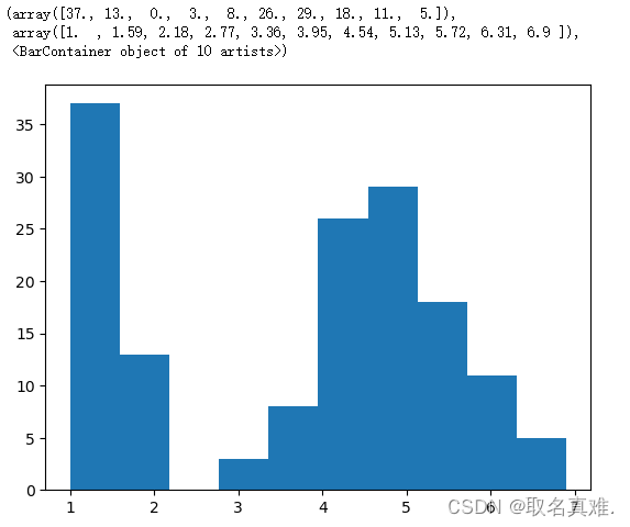
plt.hist(df_setosa['petal_length'])#柱状图
plt.hist(df_versicolor['petal_length'])
plt.hist(df_virginica['petal_length']) 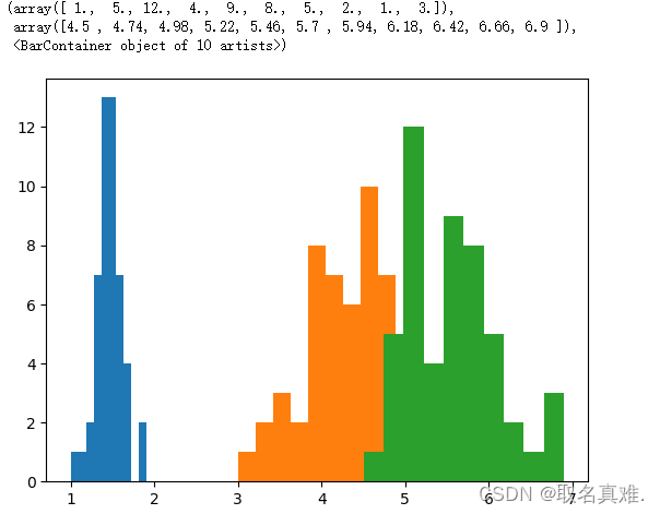
sns.distplot(df_setosa['petal_length'])
sns.distplot(df_versicolor['petal_length'])
sns.distplot(df_virginica['petal_length']) 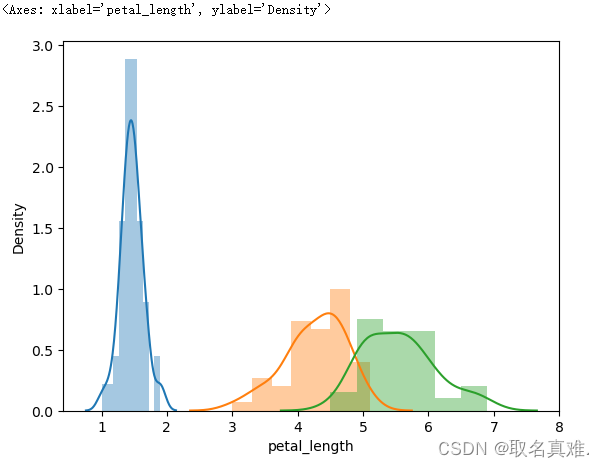
三、双变量分析
plt.plot(df_setosa['petal_length'],df_setosa["petal_width"],'o')#双变量分析
plt.plot(df_versicolor['petal_length'],df_versicolor["petal_width"],'*')
plt.plot(df_virginica['petal_length'],df_virginica["petal_width"],'x')
plt.ylabel('petal_length')
plt.show()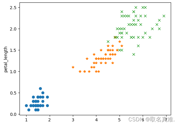
sns.FacetGrid(df,hue="species",height=5).map(plt.scatter,"petal_length","sepal_width").add_legend() 
四、多变量分析
sns.pairplot(df,hue="species",height=3)#多变量分析,变量多了在一个图表示显得凌乱,不好分析,所有采用多个图,二维的方式进行比较分析 
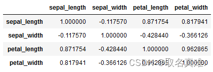
df.corr()#相关性