机器学习(Andrew Ng)作业代码(Exercise 4~)

Programming Exercise 4: Neural Networks Learning

带正则化的两层MLP,损失函数为交叉熵

sigmoidGradient

直接写Sigmoid函数的导函数即可

\[Sigmoid'(x)=Sigmoid(x)(1-Sigmoid(x))\]

function g = sigmoidGradient(z)
%SIGMOIDGRADIENT returns the gradient of the sigmoid function
%evaluated at z
%   g = SIGMOIDGRADIENT(z) computes the gradient of the sigmoid function
%   evaluated at z. This should work regardless if z is a matrix or a
%   vector. In particular, if z is a vector or matrix, you should return
%   the gradient for each element.

g = zeros(size(z));

% ====================== YOUR CODE HERE ======================
% Instructions: Compute the gradient of the sigmoid function evaluated at
%               each value of z (z can be a matrix, vector or scalar).
    g=sigmoid(z).*(1-sigmoid(z));
% =============================================================
end

nnCostFunction

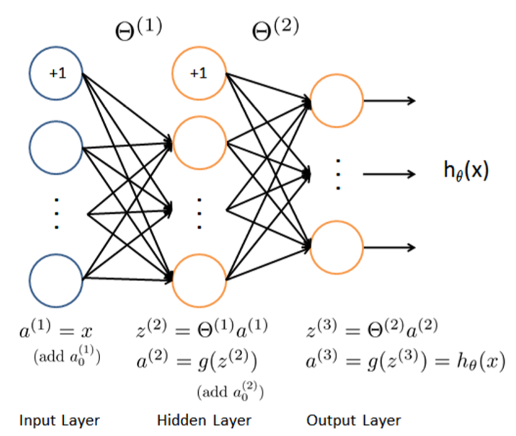
前向传播过程与Ex3一样，这里不再赘述

交叉熵损失函数

\[J(\theta)=\frac 1 m \sum_{i=1}^m\sum_{k=1}^K[-y_k^{(i)}log((h_\theta(x^{(i)}))_k)-(1-y_k^{(i)})log(1-(h_\theta(x^{(i)}))_k)]\]

\[\delta_k^{(3)}=a_k^{(3)}-y_k\]

若输入样本的真实分类为k，则\(y_k=1\)，否则为0

\[\delta^{(2)}=(\Theta^{(2)})^T\delta^{(3)}.*g'(z^{(2)})\]

\[\Delta^{l}:=\Delta^{l}+\delta^{l+1}(a^{(l)})^T\]

\(\Delta^{l}_{i,j}\)表示第l层第j个结点到第l+1层第i个结点的参数，对应m个训练样本的梯度之和

则m个样本的平均梯度可以表示为

\[\frac \partial {\partial \Theta_{ij}^{(l)}}J(\Theta)=\frac 1 m \Delta_{ij}^{(l)}\]

再给损失函数加入正则化：

\[J(\theta)=\frac 1 m \sum_{i=1}^m\sum_{k=1}^K[-y_k^{(i)}log((h_\theta(x^{(i)}))_k)-(1-y_k^{(i)})log(1-(h_\theta(x^{(i)}))_k)]+ \frac \lambda {2m}[\sum_{j=1}^{s_2}\sum_{k=1}^{s_1}(\Theta_{j,k}^{(1)})^2+\sum_{j=1}^{s_3}\sum_{k=1}^{s_2}(\Theta_{j,k}^{(2)})^2]\]

\[\frac \partial {\partial \Theta_{ij}^{(l)}}J(\Theta)=\frac 1 m \Delta_{ij}^{(l)}+\frac \lambda m \Theta_{ij}^{(l)}\]

function [J grad] = nnCostFunction(nn_params, ...
                                   input_layer_size, ...
                                   hidden_layer_size, ...
                                   num_labels, ...
                                   X, y, lambda)
%NNCOSTFUNCTION Implements the neural network cost function for a two layer
%neural network which performs classification
%   [J grad] = NNCOSTFUNCTON(nn_params, hidden_layer_size, num_labels, ...
%   X, y, lambda) computes the cost and gradient of the neural network. The
%   parameters for the neural network are "unrolled" into the vector
%   nn_params and need to be converted back into the weight matrices. 
% 
%   The returned parameter grad should be a "unrolled" vector of the
%   partial derivatives of the neural network.
%

% Reshape nn_params back into the parameters Theta1 and Theta2, the weight matrices
% for our 2 layer neural network
Theta1 = reshape(nn_params(1:hidden_layer_size * (input_layer_size + 1)), ...
                 hidden_layer_size, (input_layer_size + 1));

Theta2 = reshape(nn_params((1 + (hidden_layer_size * (input_layer_size + 1))):end), ...
                 num_labels, (hidden_layer_size + 1));

% Setup some useful variables
m = size(X, 1);
         
% You need to return the following variables correctly 
J = 0;
Theta1_grad = zeros(size(Theta1));
Theta2_grad = zeros(size(Theta2));

% ====================== YOUR CODE HERE ======================
% Instructions: You should complete the code by working through the
%               following parts.
%
% Part 1: Feedforward the neural network and return the cost in the
%         variable J. After implementing Part 1, you can verify that your
%         cost function computation is correct by verifying the cost
%         computed in ex4.m
%
% Part 2: Implement the backpropagation algorithm to compute the gradients
%         Theta1_grad and Theta2_grad. You should return the partial derivatives of
%         the cost function with respect to Theta1 and Theta2 in Theta1_grad and
%         Theta2_grad, respectively. After implementing Part 2, you can check
%         that your implementation is correct by running checkNNGradients
%
%         Note: The vector y passed into the function is a vector of labels
%               containing values from 1..K. You need to map this vector into a 
%               binary vector of 1's and 0's to be used with the neural network
%               cost function.
%
%         Hint: We recommend implementing backpropagation using a for-loop
%               over the training examples if you are implementing it for the 
%               first time.
%
% Part 3: Implement regularization with the cost function and gradients.
%
%         Hint: You can implement this around the code for
%               backpropagation. That is, you can compute the gradients for
%               the regularization separately and then add them to Theta1_grad
%               and Theta2_grad from Part 2.
%


    a1=[ones(1,m);X'];
    z2=Theta1*a1;
    a2=[ones(1,m);sigmoid(z2)];
    z3=Theta2*a2;
    a3=sigmoid(z3);
    
    for i=1:m
        for k=1:size(a3,1)
            if(y(i)==k)
                J=J-log(a3(k,i));
            else
                J=J-log(1-a3(k,i));
            end
        end
    end
    J=J/m;
    
    J=J+lambda*(sum(sum(Theta1.*Theta1))+sum(sum(Theta2.*Theta2)))/(2*m);
    
    ay=a3;
    for i=1:m
        for num=1:size(a3,1)
            if(y(i)==num)
                ay(num,i)=1;
            else
                ay(num,i)=0;
            end
        end
    end
    
    for i=1:m
        delta3=(a3(:,i)-ay(:,i));
        delta2=(Theta2'*delta3).*sigmoidGradient([1;z2(:,i)]);
        Theta2_grad=Theta2_grad+delta3*a2(:,i)';
        Theta1_grad=Theta1_grad+delta2(2:end)*a1(:,i)';
    end
    
    Theta1_grad=Theta1_grad/m;
    Theta2_grad=Theta2_grad/m;
    
    %Regularization terms
    Theta1_grad(:,2:end)=Theta1_grad(:,2:end)+(lambda/m)*Theta1(:,2:end);
    Theta2_grad(:,2:end)=Theta2_grad(:,2:end)+(lambda/m)*Theta2(:,2:end);
% -------------------------------------------------------------

% =========================================================================

% Unroll gradients
grad = [Theta1_grad(:) ; Theta2_grad(:)];
end