keras实现简略版的VGGNet并加入可调整的学习率fine tuning

VGGNet的原理部分就不细说了，具体可以看原作者paper：Very Deep Learning Convolutional Neural Networks for Large-Scale Image Recognition。

这里使用小数据集去训练，因此就是用简略版的VGGNet去实现VGG思想，使用3x3的卷积核去迭代组合形成更深的网络结构。

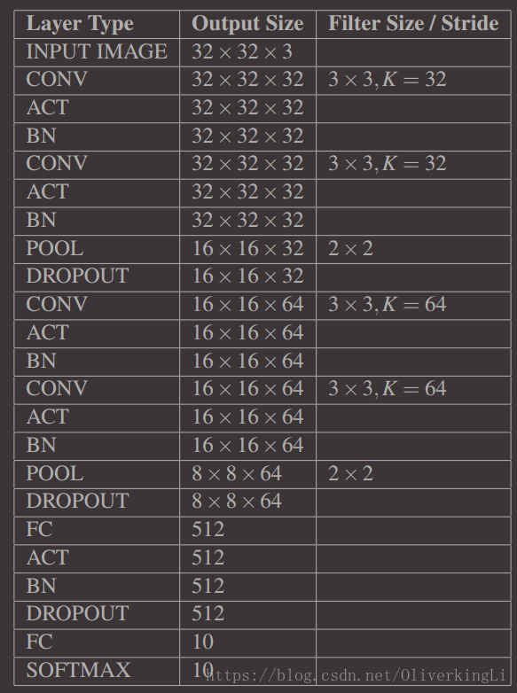
这个实现：CONV => RELU => CONV => RELU => POOL => FC => RELU => FC => SOFTMAX

定义网络结构的模块：

miniVGG.py

from keras.models import Sequential
from keras.layers.normalization import BatchNormalization
from keras.layers.convolutional import Conv2D
from keras.layers.convolutional import MaxPooling2D
from keras.layers.core import Activation, Flatten, Dropout, Dense
from keras import backend as K

class MiniVGGNet:
	@staticmethod
	def build(width, height, depth, classes):
		model = Sequential()
		inputShape = (height, width, depth)
		chanDim = -1

		if K.image_data_format() == "channels_first":
			inputShape = (depth, height, width)
			chanDim = 1

		model.add(Conv2D(32, (3, 3), padding="same", input_shape=inputShape))
		model.add(Activation("relu"))
		model.add(BatchNormalization(axis=chanDim))
		model.add(Conv2D(32, (3, 3), padding="same"))
		model.add(Activation("relu"))
		model.add(BatchNormalization(axis=chanDim))
		model.add(MaxPooling2D(pool_size=(2, 2)))
		model.add(Dropout(0.25))

		model.add(Conv2D(64, (3, 3), padding="same"))
		model.add(Activation("relu"))
		model.add(BatchNormalization(axis=chanDim))
		model.add(Conv2D(64, (3, 3), padding="same"))
		model.add(Activation("relu"))
		model.add(BatchNormalization(axis=chanDim))
		model.add(MaxPooling2D(pool_size=(2, 2)))
		model.add(Dropout(0.25))

		model.add(Flatten())
		model.add(Dense(512))
		model.add(Activation("relu"))
		model.add(BatchNormalization())
		model.add(Dropout(0.5))

		model.add(Dense(classes))
		model.add(Activation("softmax"))

		return model

这里是加入了Batch Normalization，就是进行归一化，具体也可以参考paper:Batch Normalization: Accelerating Deep Network Training by Reducing Internal Covariate Shift。

BN的作用主要是减少过拟合和提升网络的准确度，但是同时需要更多的训练epoch(时间)。

然后是训练代码：

miniVGGNetTrain.py

import matplotlib
matplotlib.use("Agg")
from sklearn.preprocessing import LabelBinarizer
from sklearn.metrics import classification_report
from miniVGG import MiniVGGNet
from keras.optimizers import SGD
from keras.callbacks import LearningRateScheduler
from keras.datasets import cifar10
from keras.datasets import cifar100
import matplotlib.pyplot as plt
import numpy as np
import argparse

ap = argparse.ArgumentParser()
ap.add_argument("-o", "--output", required=True, help="path to the output loss/accuracy plot")
ap.add_argument("-m", "--model", required=True, help="path to save train model")
args = vars(ap.parse_args())

print("[INFO] loading CIFAR-10 dataset")
((trainX, trainY), (testX, testY)) = cifar10.load_data()
trainX = trainX.astype("float") / 255.0
testX = testX.astype("float") / 255.0

lb = LabelBinarizer()
trainY = lb.fit_transform(trainY)
testY = lb.transform(testY)
# 标签0-9代表的类别string
labelNames = ['airplane', 'automobile', 'bird', 'cat', 
	'deer', 'dog', 'frog', 'horse', 'ship', 'truck']

print("[INFO] compiling model...")
opt = SGD(lr=0.01, decay=0.01 / 70, momentum=0.9, nesterov=True)
model = MiniVGGNet.build(width=32, height=32, depth=3, classes=10)
model.compile(loss="categorical_crossentropy", optimizer=opt, metrics=['accuracy'])
print(model.summary())
print("[INFO] training network Lenet-5")
H = model.fit(trainX, trainY, validation_data=(testX, testY), batch_size=64, epochs=70, 
	callbacks=callbacks, verbose=1)

model.save(args["model"])

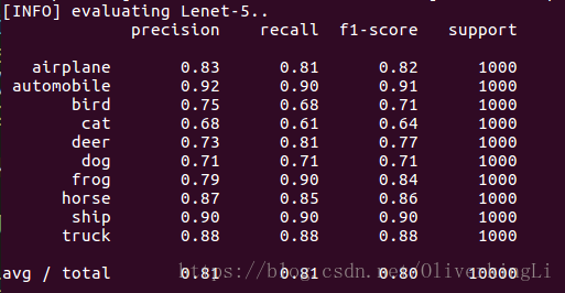
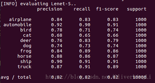
print("[INFO] evaluating Lenet-5..")
preds = model.predict(testX, batch_size=64)
print(classification_report(testY.argmax(axis=1), preds.argmax(axis=1), 
	target_names=labelNames))

# 保存可视化训练结果
plt.style.use("ggplot")
plt.figure()
plt.plot(np.arange(0, 70), H.history["loss"], label="train_loss")
plt.plot(np.arange(0, 70), H.history["val_loss"], label="val_loss")
plt.plot(np.arange(0, 70), H.history["acc"], label="train_acc")
plt.plot(np.arange(0, 70), H.history["val_acc"], label="val_acc")
plt.title("Training Loss and Accuracy")
plt.xlabel("# Epoch")
plt.ylabel("Loss/Accuracy without BatchNormalization")
plt.legend()
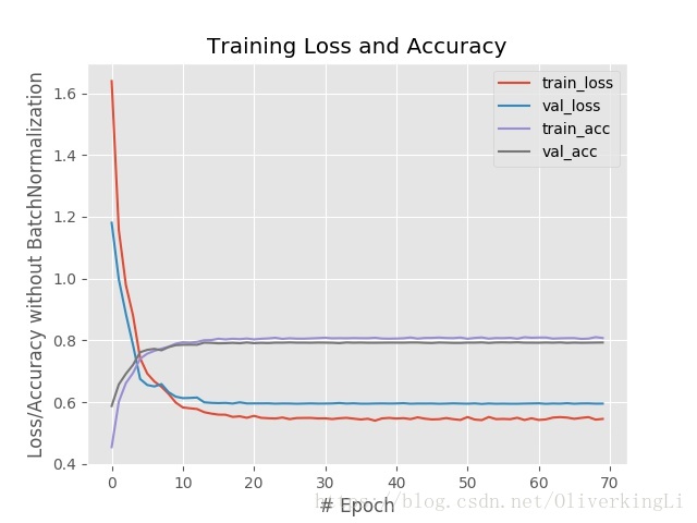
plt.savefig(args["output"])

这个是训练cifar10，代码使用的loss function的优化算法是加入开始学率0.01，每一个epoch都会相应减少0.01/epoch的大小，然后使用momentum和nesterov加速SGD梯度更新。

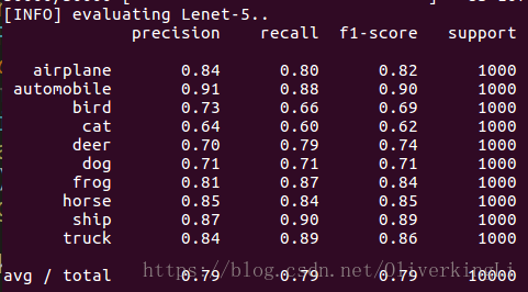
在miniVGG.py中把BN层全注释掉，然后重新训练得到没有Batch Normalization的结果：

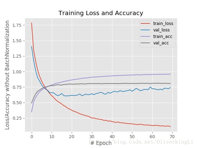
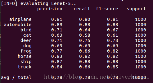
对比可以发现，BN的确可以有效的缓和过拟合，然后最终的准确度有提高，从78%提高到81%。从loss图片中看出，在加入BN后训练在到达30epoch左右出现明显过拟合（表现为validation loss的升高），而没有加入BN的时候，在训练达到20epoch时候就出现明显过拟合了，所以BN会加长模型的训练时间。

以上是加入每个epoch都会更新（减低）learning rate，现在我们使用step decay算法去更新learning rate，也就是一开始learning rate是个常数，然后经过一定的epoch后，进行更新降低，然后变为新的常熟，在经过一定的epoch后，再更新降低。使用更新公式大致如下：

新的miniVGGNetTrain.py

import matplotlib
matplotlib.use("Agg")
from sklearn.preprocessing import LabelBinarizer
from sklearn.metrics import classification_report
from miniVGG import MiniVGGNet
from keras.optimizers import SGD
from keras.callbacks import LearningRateScheduler
from keras.datasets import cifar10
from keras.datasets import cifar100
import matplotlib.pyplot as plt
import numpy as np
import argparse

def step_decay(epoch):
	initAlpha = 0.01
	factor = 0.5
	dropEvery = 5

	alpha = initAlpha * (factor ** np.floor((1 + epoch) / dropEvery))

	return float(alpha)

ap = argparse.ArgumentParser()
ap.add_argument("-o", "--output", required=True, help="path to the output loss/accuracy plot")
ap.add_argument("-m", "--model", required=True, help="path to save train model")
args = vars(ap.parse_args())

print("[INFO] loading CIFAR-10 dataset")
((trainX, trainY), (testX, testY)) = cifar10.load_data()
trainX = trainX.astype("float") / 255.0
testX = testX.astype("float") / 255.0

lb = LabelBinarizer()
trainY = lb.fit_transform(trainY)
testY = lb.transform(testY)
# 标签0-9代表的类别string
labelNames = ['airplane', 'automobile', 'bird', 'cat', 
	'deer', 'dog', 'frog', 'horse', 'ship', 'truck']

print("[INFO] compiling model...")
callbacks = [LearningRateScheduler(step_decay)]
# opt = SGD(lr=0.01, decay=0.01 / 70, momentum=0.9, nesterov=True)
opt = SGD(lr=0.01, momentum=0.9, nesterov=True)
model = MiniVGGNet.build(width=32, height=32, depth=3, classes=10)
model.compile(loss="categorical_crossentropy", optimizer=opt, metrics=['accuracy'])
print(model.summary())
print("[INFO] training network Lenet-5")
H = model.fit(trainX, trainY, validation_data=(testX, testY), batch_size=64, epochs=70, 
	callbacks=callbacks, verbose=1)

model.save(args["model"])

print("[INFO] evaluating Lenet-5..")
preds = model.predict(testX, batch_size=64)
print(classification_report(testY.argmax(axis=1), preds.argmax(axis=1), 
	target_names=labelNames))

# 保存可视化训练结果
plt.style.use("ggplot")
plt.figure()
plt.plot(np.arange(0, 70), H.history["loss"], label="train_loss")
plt.plot(np.arange(0, 70), H.history["val_loss"], label="val_loss")
plt.plot(np.arange(0, 70), H.history["acc"], label="train_acc")
plt.plot(np.arange(0, 70), H.history["val_acc"], label="val_acc")
plt.title("Training Loss and Accuracy")
plt.xlabel("# Epoch")
plt.ylabel("Loss/Accuracy without BatchNormalization")
plt.legend()
plt.savefig(args["output"])

这是F = 0.5

这是F = 0.25

F变大之后由step decay公式直到，learning rate会变得更小，然后对weight更新的贡献程度越来越小，所以对比F=0.5和F=0.25的图，F=0.5在训练接近30 epoch才出现明显的过拟合，F=0.25在15 epoch左右就出现过拟合。因此F=0.5会使得训练更稳定，可以继续进行fine tune提高准确度。

keras实现简略版的VGGNet并加入可调整的学习率fine tuning

猜你喜欢