语义分割 | 评价标准

本文为论文阅读笔记，不当之处，敬请指正。
A Review on Deep Learning Techniques Applied to Semantic Segmentation:原文链接

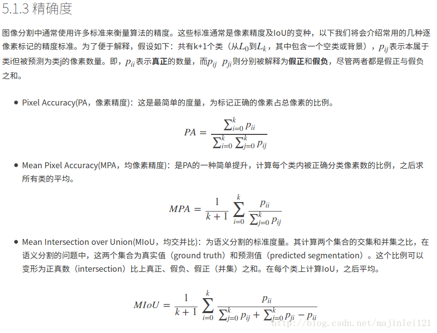
5.1度量标准

为何需要语义分割系统的评价标准？

为了衡量分割系统的作用及贡献，其性能需要经过严格评估。并且，评估须使用标准、公认的方法以保证公平性。
系统的多个方面需要被测试以评估其有效性，包括：执行时间、内存占用、和精确度。
由于系统所处背景及测试目的的不同，某些标准可能要比其他标准更加重要，例如，对于实时系统可以损失精确度以提高运算速度。而对于一种特定的方法，尽量提高所有的度量性能是必须的。

5.1.1 执行时间

速度或运行时间是一个非常有价值的度量，因为大多数系统需要保证推理时间可以满足硬实时的需求。某些情况下，知晓系统的训练时间是非常有用的，但是这通常不是非常明显，除非其特别慢。在某种意义上说，提供方法的确切时间可能不是非常有意义，因为执行时间非常依赖硬件设备及后台实现，致使一些比较是无用的。

然而，出于重用和帮助后继研究人员的目的，提供系统运行的硬件的大致描述及执行时间是有用的。这可以帮助他人评估方法的有效性，及在保证相同环境测试最快的执行方法。

5.1.2 内存占用

内存是分割方法的另一个重要的因素。尽管相比执行时间其限制较松，内存可以较为灵活地获得，但其仍然是一个约束因素。在某些情况下，如片上操作系统及机器人平台，其内存资源相比高性能服务器并不宽裕。即使是加速深度网络的高端图形处理单元（GPU），内存资源也相对有限。以此来看，在运行时间相同的情况下，记录系统运行状态下内存占用的极值和均值是及其有价值的。

深度学习之语义分割中的度量标准（准确度）(pixel accuracy, mean accuracy, mean IU, frequency weighted IU)

这里写图片描述

下面是根据全卷积语义分割的准确度程序编写

import _init_paths

import os
import numpy as np
from PIL import Image
import matplotlib.pyplot as plt
from skimage import io
from timer import Timer
import cv2
from datetime import datetime

import caffe

test_file = 'test.txt'
file_path_img = 'JPEGImages'
file_path_label = 'SegmentationClass'
save_path = 'output/results'

test_prototxt = 'Models/test.prototxt'
weight = 'Training/Seg_iter_10000.caffemodel'

layer = 'conv_seg'
save_dir = False # True

if save_dir:
    save_dir = save_path
else:
    save_dir = False

# load net
net = caffe.Net(test_prototxt, weight, caffe.TEST)

# load test.txt
test_img = np.loadtxt(test_file, dtype=str)

def fast_hist(a, b, n):
    k = (a >= 0) & (a < n)
    return np.bincount(n * a[k].astype(int) + b[k], minlength=n**2).reshape(n, n)

# seg test
print '>>>', datetime.now(), 'Begin seg tests'

n_cl = net.blobs[layer].channels
hist = np.zeros((n_cl, n_cl))

# timers
_t = {'im_seg' : Timer()}

# load image and label
i = 0
for img_name in test_img:
    _t['im_seg'].tic()
    img = Image.open(os.path.join(file_path_img, img_name + '.jpg'))
    img = img.resize((512, 384), Image.ANTIALIAS)

    in_ = np.array(img, dtype=np.float32)
    in_ = in_[:,:,::-1] # rgb to bgr
    in_ -= np.array([[[68.2117, 78.2288, 75.4916]]])#数据集平均值，根据需要修改
    in_ = in_.transpose((2,0,1))

    label = Image.open(os.path.join(file_path_label, img_name + '.png'))
    label = label.resize((512, 384), Image.ANTIALIAS)#图像大小（宽，高），根据需要修改
    label = np.array(label, dtype=np.uint8)

    # shape for input (data blob is N x C x H x W), set data
    net.blobs['data'].reshape(1, *in_.shape)
    net.blobs['data'].data[...] = in_

    net.forward()
    _t['im_seg'].toc()

    print 'im_seg: {:d}/{:d} {:.3f}s' \
          .format(i + 1, len(test_img), _t['im_seg'].average_time)
    i += 1

    hist += fast_hist(label.flatten(), net.blobs[layer].data[0].argmax(0).flatten(), n_cl)

    if save_dir:
        seg = net.blobs[layer].data[0].argmax(axis=0)
        result = np.array(img, dtype=np.uint8)
        index = np.where(seg == 1)
        for i in xrange(len(index[0])):
            result[index[0][i], index[1][i], 0] =  255
            result[index[0][i], index[1][i], 1] =  0
            result[index[0][i], index[1][i], 2] =  0
        result = Image.fromarray(result.astype(np.uint8))    
        result.save(os.path.join(save_dir, img_name + '.jpg'))        

iter = len(test_img)
# overall accuracy
acc = np.diag(hist).sum() / hist.sum()
print '>>>', datetime.now(), 'Iteration', iter, 'overall accuracy', acc
# per-class accuracy
acc = np.diag(hist) / hist.sum(1)
print '>>>', datetime.now(), 'Iteration', iter, 'mean accuracy', np.nanmean(acc)
# per-class IU
iu = np.diag(hist) / (hist.sum(1) + hist.sum(0) - np.diag(hist))
print '>>>', datetime.now(), 'Iteration', iter, 'mean IU', np.nanmean(iu)
freq = hist.sum(1) / hist.sum()
print '>>>', datetime.now(), 'Iteration', iter, 'fwavacc', \
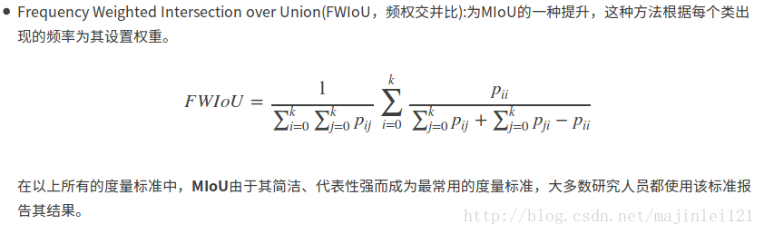
    (freq[freq > 0] * iu[freq > 0]).sum()

直观理解

如下图所示，红色圆代表真实值，黄色圆代表预测值。橙色部分红色圆与黄色圆的交集，即真正（预测为1，真实值为1）的部分，红色部分表示假负（预测为0，真实为1）的部分，黄色表示假正（预测为1，真实为0）的部分，两个圆之外的白色区域表示真负（预测为0，真实值为0）的部分。

MP计算橙色与（橙色与红色）的比例。
MIoU计算的是计算A与B的交集（橙色部分）与A与B的并集（红色+橙色+黄色）之间的比例，在理想状态下A与B重合，两者比例为1 。
参考：【1】https://blog.csdn.net/u014593748/article/details/71698246
【2】https://blog.csdn.net/majinlei121/article/details/78965435
【3】https://github.com/TqDavid/py_img_seg_eval