Part 1:Face Recognition for the Happy House
Welcome to the first assignment of week 4! Here you will build a face recognition system. Many of the ideas presented here are from FaceNet. In lecture, we also talked about DeepFace.
Face recognition problems commonly fall into two categories:
- Face Verification - “is this the claimed person?”. For example, at some airports, you can pass through customs by letting a system scan your passport and then verifying that you (the person carrying the passport) are the correct person. A mobile phone that unlocks using your face is also using face verification. This is a 1:1 matching problem.
- Face Recognition - “who is this person?”. For example, the video lecture showed a face recognition video (https://www.youtube.com/watch?v=wr4rx0Spihs) of Baidu employees entering the office without needing to otherwise identify themselves. This is a 1:K matching problem.
FaceNet learns a neural network that encodes a face image into a vector of 128 numbers. By comparing two such vectors, you can then determine if two pictures are of the same person.
In this assignment, you will:
- Implement the triplet loss function
- Use a pretrained model to map face images into 128-dimensional encodings
- Use these encodings to perform face verification and face recognition
In this exercise, we will be using a pre-trained model which represents ConvNet activations using a “channels first” convention, as opposed to the “channels last” convention used in lecture and previous programming assignments. In other words, a batch of images will be of shape (m,nC,nH,nW)(m,nC,nH,nW) instead of (m,nH,nW,nC)(m,nH,nW,nC). Both of these conventions have a reasonable amount of traction among open-source implementations; there isn’t a uniform standard yet within the deep learning community.
Let’s load the required packages.
<span style="color:#000000"><code class="language-python"><span style="color:#000088">from</span> keras.models <span style="color:#000088">import</span> Sequential
<span style="color:#000088">from</span> keras.layers <span style="color:#000088">import</span> Conv2D, ZeroPadding2D, Activation, Input, concatenate
<span style="color:#000088">from</span> keras.models <span style="color:#000088">import</span> Model
<span style="color:#000088">from</span> keras.layers.normalization <span style="color:#000088">import</span> BatchNormalization
<span style="color:#000088">from</span> keras.layers.pooling <span style="color:#000088">import</span> MaxPooling2D, AveragePooling2D
<span style="color:#000088">from</span> keras.layers.merge <span style="color:#000088">import</span> Concatenate
<span style="color:#000088">from</span> keras.layers.core <span style="color:#000088">import</span> Lambda, Flatten, Dense
<span style="color:#000088">from</span> keras.initializers <span style="color:#000088">import</span> glorot_uniform
<span style="color:#000088">from</span> keras.engine.topology <span style="color:#000088">import</span> Layer
<span style="color:#000088">from</span> keras <span style="color:#000088">import</span> backend <span style="color:#000088">as</span> K
K.set_image_data_format(<span style="color:#009900">'channels_first'</span>)
<span style="color:#000088">import</span> cv2
<span style="color:#000088">import</span> os
<span style="color:#000088">import</span> numpy <span style="color:#000088">as</span> np
<span style="color:#000088">from</span> numpy <span style="color:#000088">import</span> genfromtxt
<span style="color:#000088">import</span> pandas <span style="color:#000088">as</span> pd
<span style="color:#000088">import</span> tensorflow <span style="color:#000088">as</span> tf
<span style="color:#000088">from</span> fr_utils <span style="color:#000088">import</span> *
<span style="color:#000088">from</span> inception_blocks_v2 <span style="color:#000088">import</span> *

%matplotlib inline
%load_ext autoreload
%autoreload <span style="color:#006666">2</span>

np.set_printoptions(threshold=np.nan)</code></span>
You can get the data sets and other functions from here:https://pan.baidu.com/s/1boZGtcj 。
0 - Naive Face Verification
In Face Verification, you’re given two images and you have to tell if they are of the same person. The simplest way to do this is to compare the two images pixel-by-pixel. If the distance between the raw images are less than a chosen threshold, it may be the same person!
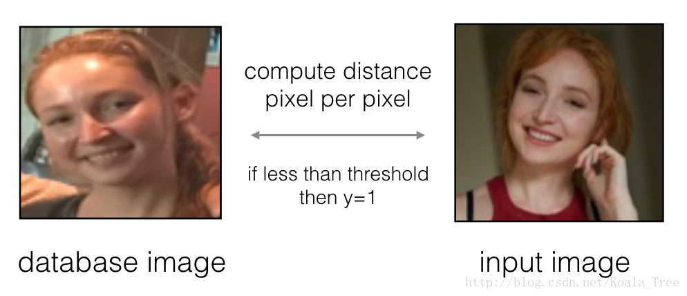
Figure 1
Of course, this algorithm performs really poorly, since the pixel values change dramatically due to variations in lighting, orientation of the person’s face, even minor changes in head position, and so on.
You’ll see that rather than using the raw image, you can learn an encoding f(img)f(img) so that element-wise comparisons of this encoding gives more accurate judgements as to whether two pictures are of the same person.
1 - Encoding face images into a 128-dimensional vector
1.1 - Using an ConvNet to compute encodings
The FaceNet model takes a lot of data and a long time to train. So following common practice in applied deep learning settings, let’s just load weights that someone else has already trained. The network architecture follows the Inception model from Szegedy et al.. We have provided an inception network implementation. You can look in the file inception_blocks.py to see how it is implemented (do so by going to “File->Open…” at the top of the Jupyter notebook).
The key things you need to know are:
- This network uses 96x96 dimensional RGB images as its input. Specifically, inputs a face image (or batch of mm face images) as a tensor of shape (m,nC,nH,nW)=(m,3,96,96)(m,nC,nH,nW)=(m,3,96,96)
- It outputs a matrix of shape (m,128)(m,128) that encodes each input face image into a 128-dimensional vector
Run the cell below to create the model for face images.
<span style="color:#000000"><code class="language-python">FRmodel = faceRecoModel(input_shape=(<span style="color:#006666">3</span>, <span style="color:#006666">96</span>, <span style="color:#006666">96</span>))</code></span><span style="color:#000000"><code class="language-python">print(<span style="color:#009900">"Total Params:"</span>, FRmodel.count_params())</code></span><span style="color:#000000"><code>Total Params: 3743280
</code></span>By using a 128-neuron fully connected layer as its last layer, the model ensures that the output is an encoding vector of size 128. You then use the encodings the compare two face images as follows:
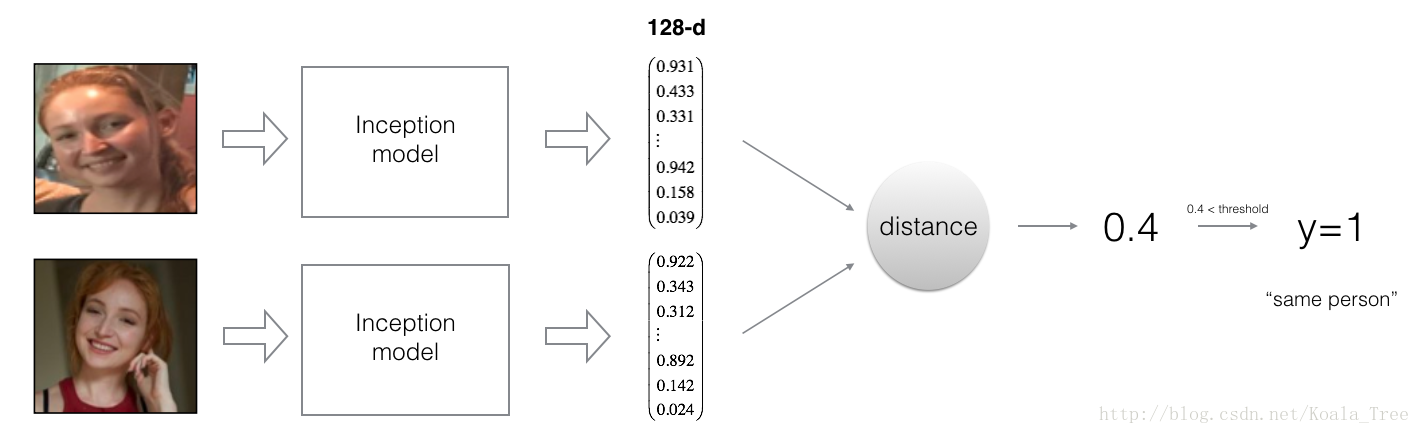
Figure 2:
By computing a distance between two encodings and thresholding, you can determine if the two pictures represent the same person
So, an encoding is a good one if:
- The encodings of two images of the same person are quite similar to each other
- The encodings of two images of different persons are very different
The triplet loss function formalizes this, and tries to “push” the encodings of two images of the same person (Anchor and Positive) closer together, while “pulling” the encodings of two images of different persons (Anchor, Negative) further apart.
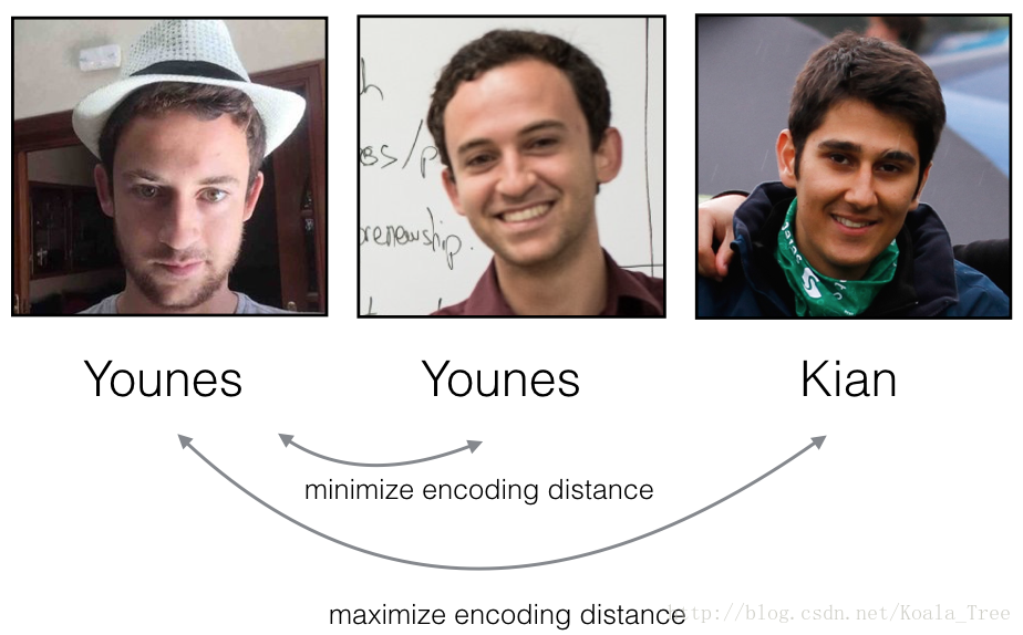
Figure 3:
In the next part, we will call the pictures from left to right: Anchor (A), Positive (P), Negative (N)
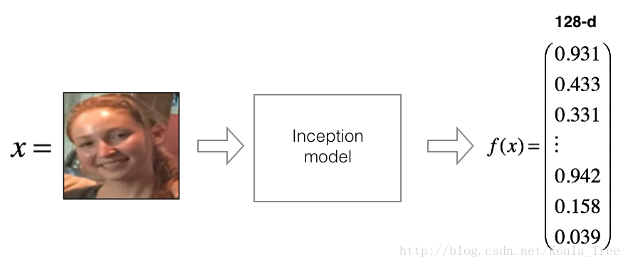
1.2 - The Triplet Loss
For an image xx, we denote its encoding f(x)f(x), where ff is the function computed by the neural network.
Training will use triplets of images (A,P,N)(A,P,N):
- A is an “Anchor” image–a picture of a person.
- P is a “Positive” image–a picture of the same person as the Anchor image.
- N is a “Negative” image–a picture of a different person than the Anchor image.
These triplets are picked from our training dataset. We will write (A(i),P(i),N(i))(A(i),P(i),N(i)) to denote the ii-th training example.
You’d like to make sure that an image A(i)A(i) of an individual is closer to the Positive P(i)P(i) than to the Negative image N(i)N(i)) by at least a margin αα:
∣∣f(A(i))−f(P(i))∣∣22+α<∣∣f(A(i))−f(N(i))∣∣22∣∣f(A(i))−f(P(i))∣∣22+α<∣∣f(A(i))−f(N(i))∣∣22
You would thus like to minimize the following “triplet cost”:
J=∑i=1m[∣∣f(A(i))−f(P(i))∣∣22(1)−∣∣f(A(i))−f(N(i))∣∣22(2)+α]+(3)(3)J=∑i=1m[∣∣f(A(i))−f(P(i))∣∣22⏟(1)−∣∣f(A(i))−f(N(i))∣∣22⏟(2)+α]+
Here, we are using the notation “[z]+[z]+” to denote max(z,0)max(z,0).
Notes:
- The term (1) is the squared distance between the anchor “A” and the positive “P” for a given triplet; you want this to be small.
- The term (2) is the squared distance between the anchor “A” and the negative “N” for a given triplet, you want this to be relatively large, so it thus makes sense to have a minus sign preceding it.
- αα is called the margin. It is a hyperparameter that you should pick manually. We will use α=0.2α=0.2.
Most implementations also normalize the encoding vectors to have norm equal one (i.e., ∣∣f(img)∣∣2∣∣f(img)∣∣2=1); you won’t have to worry about that here.
Exercise: Implement the triplet loss as defined by formula (3). Here are the 4 steps:
1. Compute the distance between the encodings of “anchor” and “positive”: ∣∣f(A(i))−f(P(i))∣∣22∣∣f(A(i))−f(P(i))∣∣22
2. Compute the distance between the encodings of “anchor” and “negative”: ∣∣f(A(i))−f(N(i))∣∣22∣∣f(A(i))−f(N(i))∣∣22
3. Compute the formula per training example: ∣∣f(A(i))−f(P(i))∣−∣∣f(A(i))−f(N(i))∣∣22+α∣∣f(A(i))−f(P(i))∣−∣∣f(A(i))−f(N(i))∣∣22+α
3. Compute the full formula by taking the max with zero and summing over the training examples:
J=∑i=1m[∣∣f(A(i))−f(P(i))∣∣22−∣∣f(A(i))−f(N(i))∣∣22+α]+(3)(3)J=∑i=1m[∣∣f(A(i))−f(P(i))∣∣22−∣∣f(A(i))−f(N(i))∣∣22+α]+
Useful functions: tf.reduce_sum(), tf.square(), tf.subtract(), tf.add(), tf.maximum().
For steps 1 and 2, you will need to sum over the entries of ∣∣f(A(i))−f(P(i))∣∣22∣∣f(A(i))−f(P(i))∣∣22 and ∣∣f(A(i))−f(N(i))∣∣22∣∣f(A(i))−f(N(i))∣∣22 while for step 4 you will need to sum over the training examples.
<span style="color:#000000"><code class="language-python"><span style="color:#880000"># GRADED FUNCTION: triplet_loss</span>

<span style="color:#000088">def</span> <span style="color:#009900">triplet_loss</span><span style="color:#4f4f4f">(y_true, y_pred, alpha = <span style="color:#006666">0.2</span>)</span>:
    <span style="color:#009900">"""
    Implementation of the triplet loss as defined by formula (3)

    Arguments:
    y_true -- true labels, required when you define a loss in Keras, you don't need it in this function.
    y_pred -- python list containing three objects:
            anchor -- the encodings for the anchor images, of shape (None, 128)
            positive -- the encodings for the positive images, of shape (None, 128)
            negative -- the encodings for the negative images, of shape (None, 128)

    Returns:
    loss -- real number, value of the loss
    """</span>

    anchor, positive, negative = y_pred[<span style="color:#006666">0</span>], y_pred[<span style="color:#006666">1</span>], y_pred[<span style="color:#006666">2</span>]

    <span style="color:#880000">### START CODE HERE ### (≈ 4 lines)</span>
    <span style="color:#880000"># Step 1: Compute the (encoding) distance between the anchor and the positive, you will need to sum over axis=-1</span>
    pos_dist = tf.reduce_sum(tf.square(tf.subtract(anchor, positive)))
    <span style="color:#880000"># Step 2: Compute the (encoding) distance between the anchor and the negative, you will need to sum over axis=-1</span>
    neg_dist = tf.reduce_sum(tf.square(tf.subtract(anchor, negative)))
    <span style="color:#880000"># Step 3: subtract the two previous distances and add alpha.</span>
    basic_loss = tf.add(tf.subtract(pos_dist,neg_dist), alpha)
    <span style="color:#880000"># Step 4: Take the maximum of basic_loss and 0.0. Sum over the training examples.</span>
    loss = tf.reduce_sum(tf.maximum(basic_loss, <span style="color:#006666">0.</span>))
    <span style="color:#880000">### END CODE HERE ###</span>

    <span style="color:#000088">return</span> loss</code></span>
<span style="color:#000000"><code class="language-python"><span style="color:#000088">with</span> tf.Session() <span style="color:#000088">as</span> test:
tf.set_random_seed(<span style="color:#006666">1</span>)
y_true = (<span style="color:#000088">None</span>, <span style="color:#000088">None</span>, <span style="color:#000088">None</span>)
y_pred = (tf.random_normal([<span style="color:#006666">3</span>, <span style="color:#006666">128</span>], mean=<span style="color:#006666">6</span>, stddev=<span style="color:#006666">0.1</span>, seed = <span style="color:#006666">1</span>),
tf.random_normal([<span style="color:#006666">3</span>, <span style="color:#006666">128</span>], mean=<span style="color:#006666">1</span>, stddev=<span style="color:#006666">1</span>, seed = <span style="color:#006666">1</span>),
tf.random_normal([<span style="color:#006666">3</span>, <span style="color:#006666">128</span>], mean=<span style="color:#006666">3</span>, stddev=<span style="color:#006666">4</span>, seed = <span style="color:#006666">1</span>))
loss = triplet_loss(y_true, y_pred)
print(<span style="color:#009900">"loss = "</span> + str(loss.eval()))</code></span><span style="color:#000000"><code>loss = 350.026
</code></span>2 - Loading the trained model
FaceNet is trained by minimizing the triplet loss. But since training requires a lot of data and a lot of computation, we won’t train it from scratch here. Instead, we load a previously trained model. Load a model using the following cell; this might take a couple of minutes to run.
<span style="color:#000000"><code class="language-python">FRmodel.compile(optimizer = <span style="color:#009900">'adam'</span>, loss = triplet_loss, metrics = [<span style="color:#009900">'accuracy'</span>])
load_weights_from_FaceNet(FRmodel)</code></span>
Here’re some examples of distances between the encodings between three individuals:

Figure 4:
Example of distance outputs between three individuals’ encodings
Let’s now use this model to perform face verification and face recognition!
3 - Applying the model
Back to the Happy House! Residents are living blissfully since you implemented happiness recognition for the house in an earlier assignment.
However, several issues keep coming up: The Happy House became so happy that every happy person in the neighborhood is coming to hang out in your living room. It is getting really crowded, which is having a negative impact on the residents of the house. All these random happy people are also eating all your food.
So, you decide to change the door entry policy, and not just let random happy people enter anymore, even if they are happy! Instead, you’d like to build a Face verification system so as to only let people from a specified list come in. To get admitted, each person has to swipe an ID card (identification card) to identify themselves at the door. The face recognition system then checks that they are who they claim to be.
3.1 - Face Verification
Let’s build a database containing one encoding vector for each person allowed to enter the happy house. To generate the encoding we use img_to_encoding(image_path, model) which basically runs the forward propagation of the model on the specified image.
Run the following code to build the database (represented as a python dictionary). This database maps each person’s name to a 128-dimensional encoding of their face.
<span style="color:#000000"><code class="language-python">database = {}
database[<span style="color:#009900">"danielle"</span>] = img_to_encoding(<span style="color:#009900">"images/danielle.png"</span>, FRmodel)
database[<span style="color:#009900">"younes"</span>] = img_to_encoding(<span style="color:#009900">"images/younes.jpg"</span>, FRmodel)
database[<span style="color:#009900">"tian"</span>] = img_to_encoding(<span style="color:#009900">"images/tian.jpg"</span>, FRmodel)
database[<span style="color:#009900">"andrew"</span>] = img_to_encoding(<span style="color:#009900">"images/andrew.jpg"</span>, FRmodel)
database[<span style="color:#009900">"kian"</span>] = img_to_encoding(<span style="color:#009900">"images/kian.jpg"</span>, FRmodel)
database[<span style="color:#009900">"dan"</span>] = img_to_encoding(<span style="color:#009900">"images/dan.jpg"</span>, FRmodel)
database[<span style="color:#009900">"sebastiano"</span>] = img_to_encoding(<span style="color:#009900">"images/sebastiano.jpg"</span>, FRmodel)
database[<span style="color:#009900">"bertrand"</span>] = img_to_encoding(<span style="color:#009900">"images/bertrand.jpg"</span>, FRmodel)
database[<span style="color:#009900">"kevin"</span>] = img_to_encoding(<span style="color:#009900">"images/kevin.jpg"</span>, FRmodel)
database[<span style="color:#009900">"felix"</span>] = img_to_encoding(<span style="color:#009900">"images/felix.jpg"</span>, FRmodel)
database[<span style="color:#009900">"benoit"</span>] = img_to_encoding(<span style="color:#009900">"images/benoit.jpg"</span>, FRmodel)
database[<span style="color:#009900">"arnaud"</span>] = img_to_encoding(<span style="color:#009900">"images/arnaud.jpg"</span>, FRmodel)</code></span>
Now, when someone shows up at your front door and swipes their ID card (thus giving you their name), you can look up their encoding in the database, and use it to check if the person standing at the front door matches the name on the ID.
Exercise: Implement the verify() function which checks if the front-door camera picture (image_path) is actually the person called “identity”. You will have to go through the following steps:
1. Compute the encoding of the image from image_path
2. Compute the distance about this encoding and the encoding of the identity image stored in the database
3. Open the door if the distance is less than 0.7, else do not open.
As presented above, you should use the L2 distance (np.linalg.norm). (Note: In this implementation, compare the L2 distance, not the square of the L2 distance, to the threshold 0.7.)
<span style="color:#000000"><code class="language-python"><span style="color:#880000"># GRADED FUNCTION: verify</span>

<span style="color:#000088">def</span> <span style="color:#009900">verify</span><span style="color:#4f4f4f">(image_path, identity, database, model)</span>:
    <span style="color:#009900">"""
    Function that verifies if the person on the "image_path" image is "identity".

    Arguments:
    image_path -- path to an image
    identity -- string, name of the person you'd like to verify the identity. Has to be a resident of the Happy house.
    database -- python dictionary mapping names of allowed people's names (strings) to their encodings (vectors).
    model -- your Inception model instance in Keras

    Returns:
    dist -- distance between the image_path and the image of "identity" in the database.
    door_open -- True, if the door should open. False otherwise.
    """</span>

    <span style="color:#880000">### START CODE HERE ###</span>

    <span style="color:#880000"># Step 1: Compute the encoding for the image. Use img_to_encoding() see example above. (≈ 1 line)</span>
    encoding = img_to_encoding(image_path, model)

    <span style="color:#880000"># Step 2: Compute distance with identity's image (≈ 1 line)</span>
    dist = np.linalg.norm(encoding - database[identity])

    <span style="color:#880000"># Step 3: Open the door if dist < 0.7, else don't open (≈ 3 lines)</span>
    <span style="color:#000088">if</span> dist < <span style="color:#006666">0.7</span>:
        print(<span style="color:#009900">"It's "</span> + str(identity) + <span style="color:#009900">", welcome home!"</span>)
        door_open = <span style="color:#000088">True</span>
    <span style="color:#000088">else</span>:
        print(<span style="color:#009900">"It's not "</span> + str(identity) + <span style="color:#009900">", please go away"</span>)
        door_open = <span style="color:#000088">False</span>

    <span style="color:#880000">### END CODE HERE ###</span>

    <span style="color:#000088">return</span> dist, door_open</code></span>
Younes is trying to enter the Happy House and the camera takes a picture of him (“images/camera_0.jpg”). Let’s run your verification algorithm on this picture:

<span style="color:#000000"><code class="language-python">verify(<span style="color:#009900">"images/camera_0.jpg"</span>, <span style="color:#009900">"younes"</span>, database, FRmodel)</code></span><span style="color:#000000"><code>It's younes, welcome home!
(0.65939283, True)
</code></span>Benoit, who broke the aquarium last weekend, has been banned from the house and removed from the database. He stole Kian’s ID card and came back to the house to try to present himself as Kian. The front-door camera took a picture of Benoit (“images/camera_2.jpg). Let’s run the verification algorithm to check if benoit can enter.

<span style="color:#000000"><code class="language-python">verify(<span style="color:#009900">"images/camera_2.jpg"</span>, <span style="color:#009900">"kian"</span>, database, FRmodel)</code></span><span style="color:#000000"><code>It's not kian, please go away
(0.86224014, False)
</code></span>3.2 - Face Recognition
Your face verification system is mostly working well. But since Kian got his ID card stolen, when he came back to the house that evening he couldn’t get in!
To reduce such shenanigans, you’d like to change your face verification system to a face recognition system. This way, no one has to carry an ID card anymore. An authorized person can just walk up to the house, and the front door will unlock for them!
You’ll implement a face recognition system that takes as input an image, and figures out if it is one of the authorized persons (and if so, who). Unlike the previous face verification system, we will no longer get a person’s name as another input.
Exercise: Implement who_is_it(). You will have to go through the following steps:
1. Compute the target encoding of the image from image_path
2. Find the encoding from the database that has smallest distance with the target encoding.
- Initialize the min_dist variable to a large enough number (100). It will help you keep track of what is the closest encoding to the input’s encoding.
- Loop over the database dictionary’s names and encodings. To loop use for (name, db_enc) in database.items().
- Compute L2 distance between the target “encoding” and the current “encoding” from the database.
- If this distance is less than the min_dist, then set min_dist to dist, and identity to name.
<span style="color:#000000"><code class="language-python"><span style="color:#880000"># GRADED FUNCTION: who_is_it</span>

<span style="color:#000088">def</span> <span style="color:#009900">who_is_it</span><span style="color:#4f4f4f">(image_path, database, model)</span>:
    <span style="color:#009900">"""
    Implements face recognition for the happy house by finding who is the person on the image_path image.

    Arguments:
    image_path -- path to an image
    database -- database containing image encodings along with the name of the person on the image
    model -- your Inception model instance in Keras

    Returns:
    min_dist -- the minimum distance between image_path encoding and the encodings from the database
    identity -- string, the name prediction for the person on image_path
    """</span>

    <span style="color:#880000">### START CODE HERE ### </span>

    <span style="color:#880000">## Step 1: Compute the target "encoding" for the image. Use img_to_encoding() see example above. ## (≈ 1 line)</span>
    encoding = img_to_encoding(image_path, model)

    <span style="color:#880000">## Step 2: Find the closest encoding ##</span>

    <span style="color:#880000"># Initialize "min_dist" to a large value, say 100 (≈1 line)</span>
    min_dist = <span style="color:#006666">100</span>

    <span style="color:#880000"># Loop over the database dictionary's names and encodings.</span>
    <span style="color:#000088">for</span> (name, db_enc) <span style="color:#000088">in</span> database.items():

        <span style="color:#880000"># Compute L2 distance between the target "encoding" and the current "emb" from the database. (≈ 1 line)</span>
        dist = np.linalg.norm(encoding - db_enc)

        <span style="color:#880000"># If this distance is less than the min_dist, then set min_dist to dist, and identity to name. (≈ 3 lines)</span>
        <span style="color:#000088">if</span> dist < min_dist:
            min_dist = dist
            identity = name

    <span style="color:#880000">### END CODE HERE ###</span>

    <span style="color:#000088">if</span> min_dist > <span style="color:#006666">0.7</span>:
        print(<span style="color:#009900">"Not in the database."</span>)
    <span style="color:#000088">else</span>:
        <span style="color:#000088">print</span> (<span style="color:#009900">"it's "</span> + str(identity) + <span style="color:#009900">", the distance is "</span> + str(min_dist))

    <span style="color:#000088">return</span> min_dist, identity</code></span>
Younes is at the front-door and the camera takes a picture of him (“images/camera_0.jpg”). Let’s see if your who_it_is() algorithm identifies Younes.
<span style="color:#000000"><code class="language-python">who_is_it(<span style="color:#009900">"images/camera_0.jpg"</span>, database, FRmodel)</code></span><span style="color:#000000"><code>it's younes, the distance is 0.659393
(0.65939283, 'younes')
</code></span>You can change “camera_0.jpg” (picture of younes) to “camera_1.jpg” (picture of bertrand) and see the result.
Your Happy House is running well. It only lets in authorized persons, and people don’t need to carry an ID card around anymore!
You’ve now seen how a state-of-the-art face recognition system works.
Although we won’t implement it here, here’re some ways to further improve the algorithm:
- Put more images of each person (under different lighting conditions, taken on different days, etc.) into the database. Then given a new image, compare the new face to multiple pictures of the person. This would increae accuracy.
- Crop the images to just contain the face, and less of the “border” region around the face. This preprocessing removes some of the irrelevant pixels around the face, and also makes the algorithm more robust.
What you should remember:
- Face verification solves an easier 1:1 matching problem; face recognition addresses a harder 1:K matching problem.
- The triplet loss is an effective loss function for training a neural network to learn an encoding of a face image.
- The same encoding can be used for verification and recognition. Measuring distances between two images’ encodings allows you to determine whether they are pictures of the same person.
Congrats on finishing this assignment!
References:
- Florian Schroff, Dmitry Kalenichenko, James Philbin (2015). FaceNet: A Unified Embedding for Face Recognition and Clustering
- Yaniv Taigman, Ming Yang, Marc’Aurelio Ranzato, Lior Wolf (2014). DeepFace: Closing the gap to human-level performance in face verification
- The pretrained model we use is inspired by Victor Sy Wang’s implementation and was loaded using his code: https://github.com/iwantooxxoox/Keras-OpenFace.
- Our implementation also took a lot of inspiration from the official FaceNet github repository: https://github.com/davidsandberg/facenet
Part 2:Deep Learning & Art: Neural Style Transfer
Welcome to the second assignment of this week. In this assignment, you will learn about Neural Style Transfer. This algorithm was created by Gatys et al. (2015) (https://arxiv.org/abs/1508.06576).
In this assignment, you will:
- Implement the neural style transfer algorithm
- Generate novel artistic images using your algorithm
Most of the algorithms you’ve studied optimize a cost function to get a set of parameter values. In Neural Style Transfer, you’ll optimize a cost function to get pixel values!
<span style="color:#000000"><code class="language-python"><span style="color:#000088">import</span> os
<span style="color:#000088">import</span> sys
<span style="color:#000088">import</span> scipy.io
<span style="color:#000088">import</span> scipy.misc
<span style="color:#000088">import</span> matplotlib.pyplot <span style="color:#000088">as</span> plt
<span style="color:#000088">from</span> matplotlib.pyplot <span style="color:#000088">import</span> imshow
<span style="color:#000088">from</span> PIL <span style="color:#000088">import</span> Image
<span style="color:#000088">from</span> nst_utils <span style="color:#000088">import</span> *
<span style="color:#000088">import</span> numpy <span style="color:#000088">as</span> np
<span style="color:#000088">import</span> tensorflow <span style="color:#000088">as</span> tf

%matplotlib inline</code></span>
You can get the data sets and other functions from here.
1 - Problem Statement
Neural Style Transfer (NST) is one of the most fun techniques in deep learning. As seen below, it merges two images, namely, a “content” image (C) and a “style” image (S), to create a “generated” image (G). The generated image G combines the “content” of the image C with the “style” of image S.
In this example, you are going to generate an image of the Louvre museum in Paris (content image C), mixed with a painting by Claude Monet, a leader of the impressionist movement (style image S).

Let’s see how you can do this.
2 - Transfer Learning
Neural Style Transfer (NST) uses a previously trained convolutional network, and builds on top of that. The idea of using a network trained on a different task and applying it to a new task is called transfer learning.
Following the original NST paper (https://arxiv.org/abs/1508.06576), we will use the VGG network. Specifically, we’ll use VGG-19, a 19-layer version of the VGG network. This model has already been trained on the very large ImageNet database, and thus has learned to recognize a variety of low level features (at the earlier layers) and high level features (at the deeper layers).
Run the following code to load parameters from the VGG model. This may take a few seconds.
<span style="color:#000000"><code class="language-python">model = load_vgg_model(<span style="color:#009900">"pretrained-model/imagenet-vgg-verydeep-19.mat"</span>)
print(model)</code></span>
<span style="color:#000000"><code>{'input': <tf.Variable 'Variable:0' shape=(1, 300, 400, 3) dtype=float32_ref>, 'conv1_1': <tf.Tensor 'Relu:0' shape=(1, 300, 400, 64) dtype=float32>, 'conv1_2': <tf.Tensor 'Relu_1:0' shape=(1, 300, 400, 64) dtype=float32>, 'avgpool1': <tf.Tensor 'AvgPool:0' shape=(1, 150, 200, 64) dtype=float32>, 'conv2_1': <tf.Tensor 'Relu_2:0' shape=(1, 150, 200, 128) dtype=float32>, 'conv2_2': <tf.Tensor 'Relu_3:0' shape=(1, 150, 200, 128) dtype=float32>, 'avgpool2': <tf.Tensor 'AvgPool_1:0' shape=(1, 75, 100, 128) dtype=float32>, 'conv3_1': <tf.Tensor 'Relu_4:0' shape=(1, 75, 100, 256) dtype=float32>, 'conv3_2': <tf.Tensor 'Relu_5:0' shape=(1, 75, 100, 256) dtype=float32>, 'conv3_3': <tf.Tensor 'Relu_6:0' shape=(1, 75, 100, 256) dtype=float32>, 'conv3_4': <tf.Tensor 'Relu_7:0' shape=(1, 75, 100, 256) dtype=float32>, 'avgpool3': <tf.Tensor 'AvgPool_2:0' shape=(1, 38, 50, 256) dtype=float32>, 'conv4_1': <tf.Tensor 'Relu_8:0' shape=(1, 38, 50, 512) dtype=float32>, 'conv4_2': <tf.Tensor 'Relu_9:0' shape=(1, 38, 50, 512) dtype=float32>, 'conv4_3': <tf.Tensor 'Relu_10:0' shape=(1, 38, 50, 512) dtype=float32>, 'conv4_4': <tf.Tensor 'Relu_11:0' shape=(1, 38, 50, 512) dtype=float32>, 'avgpool4': <tf.Tensor 'AvgPool_3:0' shape=(1, 19, 25, 512) dtype=float32>, 'conv5_1': <tf.Tensor 'Relu_12:0' shape=(1, 19, 25, 512) dtype=float32>, 'conv5_2': <tf.Tensor 'Relu_13:0' shape=(1, 19, 25, 512) dtype=float32>, 'conv5_3': <tf.Tensor 'Relu_14:0' shape=(1, 19, 25, 512) dtype=float32>, 'conv5_4': <tf.Tensor 'Relu_15:0' shape=(1, 19, 25, 512) dtype=float32>, 'avgpool5': <tf.Tensor 'AvgPool_4:0' shape=(1, 10, 13, 512) dtype=float32>}
</code></span>The model is stored in a python dictionary where each variable name is the key and the corresponding value is a tensor containing that variable’s value. To run an image through this network, you just have to feed the image to the model. In TensorFlow, you can do so using the tf.assign function. In particular, you will use the assign function like this:
<span style="color:#000000"><code class="language-python">model[<span style="color:#009900">"input"</span>].assign(image)</code></span>This assigns the image as an input to the model. After this, if you want to access the activations of a particular layer, say layer 4_2 when the network is run on this image, you would run a TensorFlow session on the correct tensor conv4_2, as follows:
<span style="color:#000000"><code class="language-python">sess.run(model[<span style="color:#009900">"conv4_2"</span>])</code></span>3 - Neural Style Transfer
We will build the NST algorithm in three steps:
- Build the content cost function Jcontent(C,G)Jcontent(C,G)
- Build the style cost function Jstyle(S,G)Jstyle(S,G)
- Put it together to get J(G)=αJcontent(C,G)+βJstyle(S,G)J(G)=αJcontent(C,G)+βJstyle(S,G).
3.1 - Computing the content cost
In our running example, the content image C will be the picture of the Louvre Museum in Paris. Run the code below to see a picture of the Louvre.
<span style="color:#000000"><code class="language-python">content_image = scipy.misc.imread(<span style="color:#009900">"images/louvre.jpg"</span>)
imshow(content_image)</code></span>
<span style="color:#000000"><code><matplotlib.image.AxesImage at 0x7f71dab9b748>
</code></span>

The content image (C) shows the Louvre museum’s pyramid surrounded by old Paris buildings, against a sunny sky with a few clouds.
* 3.1.1 - How do you ensure the generated image G matches the content of the image C?*
As we saw in lecture, the earlier (shallower) layers of a ConvNet tend to detect lower-level features such as edges and simple textures, and the later (deeper) layers tend to detect higher-level features such as more complex textures as well as object classes.
We would like the “generated” image G to have similar content as the input image C. Suppose you have chosen some layer’s activations to represent the content of an image. In practice, you’ll get the most visually pleasing results if you choose a layer in the middle of the network–neither too shallow nor too deep. (After you have finished this exercise, feel free to come back and experiment with using different layers, to see how the results vary.)
So, suppose you have picked one particular hidden layer to use. Now, set the image C as the input to the pretrained VGG network, and run forward propagation. Let a(C)a(C) be the hidden layer activations in the layer you had chosen. (In lecture, we had written this as a[l](C)a[l](C), but here we’ll drop the superscript [l][l] to simplify the notation.) This will be a nH×nW×nCnH×nW×nC tensor. Repeat this process with the image G: Set G as the input, and run forward progation. Let
a(G)a(G)
be the corresponding hidden layer activation. We will define as the content cost function as:
Jcontent(C,G)=14×nH×nW×nC∑all entries(a(C)−a(G))2(1)(1)Jcontent(C,G)=14×nH×nW×nC∑all entries(a(C)−a(G))2
Here, nH,nWnH,nW and nCnC are the height, width and number of channels of the hidden layer you have chosen, and appear in a normalization term in the cost. For clarity, note that a(C)a(C) and a(G)a(G) are the volumes corresponding to a hidden layer’s activations. In order to compute the cost Jcontent(C,G)Jcontent(C,G), it might also be convenient to unroll these 3D volumes into a 2D matrix, as shown below. (Technically this unrolling step isn’t needed to compute JcontentJcontent, but it will be good practice for when you do need to carry out a similar operation later for computing the style const JstyleJstyle.)

Exercise: Compute the “content cost” using TensorFlow.
Instructions: The 3 steps to implement this function are:
1. Retrieve dimensions from a_G:
- To retrieve dimensions from a tensor X, use: X.get_shape().as_list()
2. Unroll a_C and a_G as explained in the picture above
- If you are stuck, take a look at Hint1 and Hint2.
3. Compute the content cost:
- If you are stuck, take a look at Hint3, Hint4 and Hint5.
<span style="color:#000000"><code class="language-python"><span style="color:#880000"># GRADED FUNCTION: compute_content_cost</span>

<span style="color:#000088">def</span> <span style="color:#009900">compute_content_cost</span><span style="color:#4f4f4f">(a_C, a_G)</span>:
    <span style="color:#009900">"""
    Computes the content cost

    Arguments:
    a_C -- tensor of dimension (1, n_H, n_W, n_C), hidden layer activations representing content of the image C
    a_G -- tensor of dimension (1, n_H, n_W, n_C), hidden layer activations representing content of the image G

    Returns:
    J_content -- scalar that you compute using equation 1 above.
    """</span>

    <span style="color:#880000">### START CODE HERE ###</span>
    <span style="color:#880000"># Retrieve dimensions from a_G (≈1 line)</span>
    m, n_H, n_W, n_C = a_G.get_shape().as_list()

    <span style="color:#880000"># Reshape a_C and a_G (≈2 lines)</span>
    a_C_unrolled = tf.reshape(a_C, [n_H*n_W, n_C])
    a_G_unrolled = tf.reshape(a_G, [n_H*n_W, n_C])

    <span style="color:#880000"># compute the cost with tensorflow (≈1 line)</span>
    J_content = <span style="color:#006666">1.</span>/(<span style="color:#006666">4</span> * n_H * n_W * n_C)*tf.reduce_sum(tf.square(tf.subtract(a_C_unrolled, a_G_unrolled)))
    <span style="color:#880000">### END CODE HERE ###</span>

    <span style="color:#000088">return</span> J_content</code></span>
<span style="color:#000000"><code class="language-python">tf.reset_default_graph()
<span style="color:#000088">with</span> tf.Session() <span style="color:#000088">as</span> test:
tf.set_random_seed(<span style="color:#006666">1</span>)
a_C = tf.random_normal([<span style="color:#006666">1</span>, <span style="color:#006666">4</span>, <span style="color:#006666">4</span>, <span style="color:#006666">3</span>], mean=<span style="color:#006666">1</span>, stddev=<span style="color:#006666">4</span>)
a_G = tf.random_normal([<span style="color:#006666">1</span>, <span style="color:#006666">4</span>, <span style="color:#006666">4</span>, <span style="color:#006666">3</span>], mean=<span style="color:#006666">1</span>, stddev=<span style="color:#006666">4</span>)
J_content = compute_content_cost(a_C, a_G)
print(<span style="color:#009900">"J_content = "</span> + str(J_content.eval()))</code></span><span style="color:#000000"><code>J_content = 6.76559
</code></span>
What you should remember:
- The content cost takes a hidden layer activation of the neural network, and measures how different a(C)a(C) and a(G)a(G) are.
- When we minimize the content cost later, this will help make sure GG has similar content as CC.
3.2 - Computing the style cost
For our running example, we will use the following style image:
<span style="color:#000000"><code class="language-python">style_image = scipy.misc.imread(<span style="color:#009900">"images/monet_800600.jpg"</span>)
imshow(style_image)</code></span>
<span style="color:#000000"><code><matplotlib.image.AxesImage at 0x7f71d82a71d0>
</code></span>

This painting was painted in the style of impressionism.
Lets see how you can now define a “style” const function Jstyle(S,G)Jstyle(S,G).
3.2.1 - Style matrix
The style matrix is also called a “Gram matrix.” In linear algebra, the Gram matrix G of a set of vectors (v1,…,vn)(v1,…,vn) is the matrix of dot products, whose entries are Gij=vTivj=np.dot(vi,vj)Gij=viTvj=np.dot(vi,vj). In other words, GijGij compares how similar vivi is to vjvj: If they are highly similar, you would expect them to have a large dot product, and thus for GijGij to be large.
Note that there is an unfortunate collision in the variable names used here. We are following common terminology used in the literature, but GG is used to denote the Style matrix (or Gram matrix) as well as to denote the generated image GG. We will try to make sure which GG we are referring to is always clear from the context.
In NST, you can compute the Style matrix by multiplying the “unrolled” filter matrix with their transpose:

The result is a matrix of dimension (nC,nC)(nC,nC) where nCnC is the number of filters. The value GijGij measures how similar the activations of filter ii are to the activations of filter jj.
One important part of the gram matrix is that the diagonal elements such as GiiGii also measures how active filter ii is. For example, suppose filter ii is detecting vertical textures in the image. Then GiiGii measures how common vertical textures are in the image as a whole: If GiiGii is large, this means that the image has a lot of vertical texture.
By capturing the prevalence of different types of features (GiiGii), as well as how much different features occur together (GijGij), the Style matrix GG measures the style of an image.
Exercise:
Using TensorFlow, implement a function that computes the Gram matrix of a matrix A. The formula is: The gram matrix of A is GA=AATGA=AAT. If you are stuck, take a look at Hint 1 and Hint 2.
<span style="color:#000000"><code class="language-python"><span style="color:#880000"># GRADED FUNCTION: gram_matrix</span>

<span style="color:#000088">def</span> <span style="color:#009900">gram_matrix</span><span style="color:#4f4f4f">(A)</span>:
    <span style="color:#009900">"""
    Argument:
    A -- matrix of shape (n_C, n_H*n_W)

    Returns:
    GA -- Gram matrix of A, of shape (n_C, n_C)
    """</span>

    <span style="color:#880000">### START CODE HERE ### (≈1 line)</span>
    GA = tf.matmul(A, tf.transpose(A))
    <span style="color:#880000">### END CODE HERE ###</span>

    <span style="color:#000088">return</span> GA</code></span>
<span style="color:#000000"><code class="language-python">tf.reset_default_graph()
<span style="color:#000088">with</span> tf.Session() <span style="color:#000088">as</span> test:
tf.set_random_seed(<span style="color:#006666">1</span>)
A = tf.random_normal([<span style="color:#006666">3</span>, <span style="color:#006666">2</span>*<span style="color:#006666">1</span>], mean=<span style="color:#006666">1</span>, stddev=<span style="color:#006666">4</span>)
GA = gram_matrix(A)
print(<span style="color:#009900">"GA = "</span> + str(GA.eval()))</code></span><span style="color:#000000"><code>GA = [[ 6.42230511 -4.42912197 -2.09668207]
[ -4.42912197 19.46583748 19.56387138]
[ -2.09668207 19.56387138 20.6864624 ]]
</code></span>3.2.2 - Style cost
After generating the Style matrix (Gram matrix), your goal will be to minimize the distance between the Gram matrix of the “style” image S and that of the “generated” image G. For now, we are using only a single hidden layer a[l]a[l], and the corresponding style cost for this layer is defined as:
J[l]style(S,G)=14×nC2×(nH×nW)2∑i=1nC∑j=1nC(G(S)ij−G(G)ij)2(2)(2)Jstyle[l](S,G)=14×nC2×(nH×nW)2∑i=1nC∑j=1nC(Gij(S)−Gij(G))2
where G(S)G(S) and G(G)G(G) are respectively the Gram matrices of the “style” image and the “generated” image, computed using the hidden layer activations for a particular hidden layer in the network.
Exercise: Compute the style cost for a single layer.
Instructions: The 3 steps to implement this function are:
1. Retrieve dimensions from the hidden layer activations a_G:
- To retrieve dimensions from a tensor X, use: X.get_shape().as_list()
2. Unroll the hidden layer activations a_S and a_G into 2D matrices, as explained in the picture above.
- You may find Hint1 and Hint2 useful.
3. Compute the Style matrix of the images S and G. (Use the function you had previously written.)
4. Compute the Style cost:
- You may find Hint3, Hint4 and Hint5 useful.
<span style="color:#000000"><code class="language-python"><span style="color:#880000"># GRADED FUNCTION: compute_layer_style_cost</span>

<span style="color:#000088">def</span> <span style="color:#009900">compute_layer_style_cost</span><span style="color:#4f4f4f">(a_S, a_G)</span>:
    <span style="color:#009900">"""
    Arguments:
    a_S -- tensor of dimension (1, n_H, n_W, n_C), hidden layer activations representing style of the image S
    a_G -- tensor of dimension (1, n_H, n_W, n_C), hidden layer activations representing style of the image G

    Returns:
    J_style_layer -- tensor representing a scalar value, style cost defined above by equation (2)
    """</span>

    <span style="color:#880000">### START CODE HERE ###</span>
    <span style="color:#880000"># Retrieve dimensions from a_G (≈1 line)</span>
    m, n_H, n_W, n_C = a_G.get_shape().as_list()

    <span style="color:#880000"># Reshape the images to have them of shape (n_C, n_H*n_W) (≈2 lines)</span>
    a_S = tf.transpose(tf.reshape(a_S, [n_H*n_W, n_C]))
    a_G = tf.transpose(tf.reshape(a_G, [n_H*n_W, n_C]))

    <span style="color:#880000"># Computing gram_matrices for both images S and G (≈2 lines)</span>
    GS = gram_matrix(a_S)
    GG = gram_matrix(a_G)

    <span style="color:#880000"># Computing the loss (≈1 line)</span>
    J_style_layer = <span style="color:#006666">1.</span>/(<span style="color:#006666">4</span> * n_C * n_C * n_H * n_W * n_H * n_W) * tf.reduce_sum(tf.square(tf.subtract(GS, GG)))

    <span style="color:#880000">### END CODE HERE ###</span>

    <span style="color:#000088">return</span> J_style_layer</code></span>
<span style="color:#000000"><code class="language-python">tf.reset_default_graph()
<span style="color:#000088">with</span> tf.Session() <span style="color:#000088">as</span> test:
tf.set_random_seed(<span style="color:#006666">1</span>)
a_S = tf.random_normal([<span style="color:#006666">1</span>, <span style="color:#006666">4</span>, <span style="color:#006666">4</span>, <span style="color:#006666">3</span>], mean=<span style="color:#006666">1</span>, stddev=<span style="color:#006666">4</span>)
a_G = tf.random_normal([<span style="color:#006666">1</span>, <span style="color:#006666">4</span>, <span style="color:#006666">4</span>, <span style="color:#006666">3</span>], mean=<span style="color:#006666">1</span>, stddev=<span style="color:#006666">4</span>)
J_style_layer = compute_layer_style_cost(a_S, a_G)
print(<span style="color:#009900">"J_style_layer = "</span> + str(J_style_layer.eval()))</code></span><span style="color:#000000"><code>J_style_layer = 9.19028
</code></span>3.2.3 Style Weights
So far you have captured the style from only one layer. We’ll get better results if we “merge” style costs from several different layers. After completing this exercise, feel free to come back and experiment with different weights to see how it changes the generated image GG. But for now, this is a pretty reasonable default:
<span style="color:#000000"><code class="language-python">STYLE_LAYERS = [
    (<span style="color:#009900">'conv1_1'</span>, <span style="color:#006666">0.2</span>),
    (<span style="color:#009900">'conv2_1'</span>, <span style="color:#006666">0.2</span>),
    (<span style="color:#009900">'conv3_1'</span>, <span style="color:#006666">0.2</span>),
    (<span style="color:#009900">'conv4_1'</span>, <span style="color:#006666">0.2</span>),
    (<span style="color:#009900">'conv5_1'</span>, <span style="color:#006666">0.2</span>)]</code></span>
You can combine the style costs for different layers as follows:
Jstyle(S,G)=∑lλ[l]J[l]style(S,G)Jstyle(S,G)=∑lλ[l]Jstyle[l](S,G)
where the values for λ[l]λ[l] are given in STYLE_LAYERS.
We’ve implemented a compute_style_cost(…) function. It simply calls your compute_layer_style_cost(...) several times, and weights their results using the values in STYLE_LAYERS. Read over it to make sure you understand what it’s doing.
<span style="color:#000000"><code class="language-python"><span style="color:#000088">def</span> <span style="color:#009900">compute_style_cost</span><span style="color:#4f4f4f">(model, STYLE_LAYERS)</span>:
    <span style="color:#009900">"""
    Computes the overall style cost from several chosen layers

    Arguments:
    model -- our tensorflow model
    STYLE_LAYERS -- A python list containing:
                        - the names of the layers we would like to extract style from
                        - a coefficient for each of them

    Returns:
    J_style -- tensor representing a scalar value, style cost defined above by equation (2)
    """</span>

    <span style="color:#880000"># initialize the overall style cost</span>
    J_style = <span style="color:#006666">0</span>

    <span style="color:#000088">for</span> layer_name, coeff <span style="color:#000088">in</span> STYLE_LAYERS:

        <span style="color:#880000"># Select the output tensor of the currently selected layer</span>
        out = model[layer_name]

        <span style="color:#880000"># Set a_S to be the hidden layer activation from the layer we have selected, by running the session on out</span>
        a_S = sess.run(out)

        <span style="color:#880000"># Set a_G to be the hidden layer activation from same layer. Here, a_G references model[layer_name] </span>
        <span style="color:#880000"># and isn't evaluated yet. Later in the code, we'll assign the image G as the model input, so that</span>
        <span style="color:#880000"># when we run the session, this will be the activations drawn from the appropriate layer, with G as input.</span>
        a_G = out

        <span style="color:#880000"># Compute style_cost for the current layer</span>
        J_style_layer = compute_layer_style_cost(a_S, a_G)

        <span style="color:#880000"># Add coeff * J_style_layer of this layer to overall style cost</span>
        J_style += coeff * J_style_layer

<span style="color:#000088">return</span> J_style</code></span>Note: In the inner-loop of the for-loop above, a_G is a tensor and hasn’t been evaluated yet. It will be evaluated and updated at each iteration when we run the TensorFlow graph in model_nn() below.
What you should remember:
- The style of an image can be represented using the Gram matrix of a hidden layer’s activations. However, we get even better results combining this representation from multiple different layers. This is in contrast to the content representation, where usually using just a single hidden layer is sufficient.
- Minimizing the style cost will cause the image GG to follow the style of the image SS.
3.3 - Defining the total cost to optimize
Finally, let’s create a cost function that minimizes both the style and the content cost. The formula is:
J(G)=αJcontent(C,G)+βJstyle(S,G)J(G)=αJcontent(C,G)+βJstyle(S,G)
Exercise: Implement the total cost function which includes both the content cost and the style cost.
<span style="color:#000000"><code class="language-python"><span style="color:#880000"># GRADED FUNCTION: total_cost</span>

<span style="color:#000088">def</span> <span style="color:#009900">total_cost</span><span style="color:#4f4f4f">(J_content, J_style, alpha = <span style="color:#006666">10</span>, beta = <span style="color:#006666">40</span>)</span>:
    <span style="color:#009900">"""
    Computes the total cost function

    Arguments:
    J_content -- content cost coded above
    J_style -- style cost coded above
    alpha -- hyperparameter weighting the importance of the content cost
    beta -- hyperparameter weighting the importance of the style cost

    Returns:
    J -- total cost as defined by the formula above.
    """</span>

    <span style="color:#880000">### START CODE HERE ### (≈1 line)</span>
    J = alpha * J_content + beta * J_style
    <span style="color:#880000">### END CODE HERE ###</span>

    <span style="color:#000088">return</span> J</code></span>
<span style="color:#000000"><code class="language-python">tf.reset_default_graph()
<span style="color:#000088">with</span> tf.Session() <span style="color:#000088">as</span> test:
np.random.seed(<span style="color:#006666">3</span>)
J_content = np.random.randn()
J_style = np.random.randn()
J = total_cost(J_content, J_style)
print(<span style="color:#009900">"J = "</span> + str(J))</code></span><span style="color:#000000"><code>J = 35.34667875478276
</code></span>
What you should remember:
- The total cost is a linear combination of the content cost Jcontent(C,G)Jcontent(C,G) and the style cost Jstyle(S,G)Jstyle(S,G)
- αα and ββ are hyperparameters that control the relative weighting between content and style
4 - Solving the optimization problem
Finally, let’s put everything together to implement Neural Style Transfer!
Here’s what the program will have to do:
- Create an Interactive Session
- Load the content image
- Load the style image
- Randomly initialize the image to be generated
- Load the VGG16 model
- Build the TensorFlow graph:
- Run the content image through the VGG16 model and compute the content cost
- Run the style image through the VGG16 model and compute the style cost
- Compute the total cost
- Define the optimizer and the learning rate
- Initialize the TensorFlow graph and run it for a large number of iterations, updating the generated image at every step.
Lets go through the individual steps in detail.
You’ve previously implemented the overall cost J(G)J(G). We’ll now set up TensorFlow to optimize this with respect to GG. To do so, your program has to reset the graph and use an “Interactive Session“. Unlike a regular session, the “Interactive Session” installs itself as the default session to build a graph. This allows you to run variables without constantly needing to refer to the session object, which simplifies the code.
Lets start the interactive session.
<span style="color:#000000"><code class="language-python"><span style="color:#880000"># Reset the graph</span>
tf.reset_default_graph()

<span style="color:#880000"># Start interactive session</span>
sess = tf.InteractiveSession()</code></span>
Let’s load, reshape, and normalize our “content” image (the Louvre museum picture):
<span style="color:#000000"><code class="language-python">content_image = scipy.misc.imread(<span style="color:#009900">"images/louvre_small.jpg"</span>)
content_image = reshape_and_normalize_image(content_image)</code></span>
Let’s load, reshape and normalize our “style” image (Claude Monet’s painting):
<span style="color:#000000"><code class="language-python">style_image = scipy.misc.imread(<span style="color:#009900">"images/monet.jpg"</span>)
style_image = reshape_and_normalize_image(style_image)</code></span>
Now, we initialize the “generated” image as a noisy image created from the content_image. By initializing the pixels of the generated image to be mostly noise but still slightly correlated with the content image, this will help the content of the “generated” image more rapidly match the content of the “content” image. (Feel free to look in nst_utils.py to see the details of generate_noise_image(...); to do so, click “File–>Open…” at the upper-left corner of this Jupyter notebook.)
<span style="color:#000000"><code class="language-python">generated_image = generate_noise_image(content_image)
imshow(generated_image[<span style="color:#006666">0</span>])</code></span>
<span style="color:#000000"><code><matplotlib.image.AxesImage at 0x7f71d07ac6d8>
</code></span>

Next, as explained in part (2), let’s load the VGG16 model.
<span style="color:#000000"><code class="language-python">model = load_vgg_model(<span style="color:#009900">"pretrained-model/imagenet-vgg-verydeep-19.mat"</span>)</code></span>To get the program to compute the content cost, we will now assign a_C and a_G to be the appropriate hidden layer activations. We will use layer conv4_2 to compute the content cost. The code below does the following:
- Assign the content image to be the input to the VGG model.
- Set a_C to be the tensor giving the hidden layer activation for layer “conv4_2”.
- Set a_G to be the tensor giving the hidden layer activation for the same layer.
- Compute the content cost using a_C and a_G.
<span style="color:#000000"><code class="language-python"><span style="color:#880000"># Assign the content image to be the input of the VGG model.  </span>
sess.run(model[<span style="color:#009900">'input'</span>].assign(content_image))

<span style="color:#880000"># Select the output tensor of layer conv4_2</span>
out = model[<span style="color:#009900">'conv4_2'</span>]

<span style="color:#880000"># Set a_C to be the hidden layer activation from the layer we have selected</span>
a_C = sess.run(out)

<span style="color:#880000"># Set a_G to be the hidden layer activation from same layer. Here, a_G references model['conv4_2'] </span>
<span style="color:#880000"># and isn't evaluated yet. Later in the code, we'll assign the image G as the model input, so that</span>
<span style="color:#880000"># when we run the session, this will be the activations drawn from the appropriate layer, with G as input.</span>
a_G = out

<span style="color:#880000"># Compute the content cost</span>
J_content = compute_content_cost(a_C, a_G)</code></span>Note: At this point, a_G is a tensor and hasn’t been evaluated. It will be evaluated and updated at each iteration when we run the Tensorflow graph in model_nn() below.
<span style="color:#000000"><code class="language-python"><span style="color:#880000"># Assign the input of the model to be the "style" image </span>
sess.run(model[<span style="color:#009900">'input'</span>].assign(style_image))

<span style="color:#880000"># Compute the style cost</span>
J_style = compute_style_cost(model, STYLE_LAYERS)</code></span>Exercise: Now that you have J_content and J_style, compute the total cost J by calling total_cost(). Use alpha = 10 and beta = 40.
<span style="color:#000000"><code class="language-python"><span style="color:#880000">### START CODE HERE ### (1 line)</span>
J = total_cost(J_content, J_style, <span style="color:#006666">10</span>, <span style="color:#006666">40</span>)
<span style="color:#880000">### END CODE HERE ###</span></code></span>
You’d previously learned how to set up the Adam optimizer in TensorFlow. Lets do that here, using a learning rate of 2.0. See reference
<span style="color:#000000"><code class="language-python"><span style="color:#880000"># define optimizer (1 line)</span>
optimizer = tf.train.AdamOptimizer(<span style="color:#006666">2.0</span>)

<span style="color:#880000"># define train_step (1 line)</span>
train_step = optimizer.minimize(J)</code></span>Exercise: Implement the model_nn() function which initializes the variables of the tensorflow graph, assigns the input image (initial generated image) as the input of the VGG16 model and runs the train_step for a large number of steps.
<span style="color:#000000"><code class="language-python"><span style="color:#000088">def</span> <span style="color:#009900">model_nn</span><span style="color:#4f4f4f">(sess, input_image, num_iterations = <span style="color:#006666">200</span>)</span>:

    <span style="color:#880000"># Initialize global variables (you need to run the session on the initializer)</span>
    <span style="color:#880000">### START CODE HERE ### (1 line)</span>
    sess.run(tf.global_variables_initializer())
    <span style="color:#880000">### END CODE HERE ###</span>

    <span style="color:#880000"># Run the noisy input image (initial generated image) through the model. Use assign().</span>
    <span style="color:#880000">### START CODE HERE ### (1 line)</span>
    sess.run(model[<span style="color:#009900">"input"</span>].assign(input_image))
    <span style="color:#880000">### END CODE HERE ###</span>

    <span style="color:#000088">for</span> i <span style="color:#000088">in</span> range(num_iterations):

        <span style="color:#880000"># Run the session on the train_step to minimize the total cost</span>
        <span style="color:#880000">### START CODE HERE ### (1 line)</span>
        sess.run(train_step)
        <span style="color:#880000">### END CODE HERE ###</span>

        <span style="color:#880000"># Compute the generated image by running the session on the current model['input']</span>
        <span style="color:#880000">### START CODE HERE ### (1 line)</span>
        generated_image =sess.run(model[<span style="color:#009900">"input"</span>])
        <span style="color:#880000">### END CODE HERE ###</span>

        <span style="color:#880000"># Print every 20 iteration.</span>
        <span style="color:#000088">if</span> i%<span style="color:#006666">20</span> == <span style="color:#006666">0</span>:
            Jt, Jc, Js = sess.run([J, J_content, J_style])
            print(<span style="color:#009900">"Iteration "</span> + str(i) + <span style="color:#009900">" :"</span>)
            print(<span style="color:#009900">"total cost = "</span> + str(Jt))
            print(<span style="color:#009900">"content cost = "</span> + str(Jc))
            print(<span style="color:#009900">"style cost = "</span> + str(Js))

            <span style="color:#880000"># save current generated image in the "/output" directory</span>
            save_image(<span style="color:#009900">"output/"</span> + str(i) + <span style="color:#009900">".png"</span>, generated_image)

    <span style="color:#880000"># save last generated image</span>
    save_image(<span style="color:#009900">'output/generated_image.jpg'</span>, generated_image)

    <span style="color:#000088">return</span> generated_image</code></span>
Run the following cell to generate an artistic image. It should take about 3min on CPU for every 20 iterations but you start observing attractive results after ≈140 iterations. Neural Style Transfer is generally trained using GPUs.
<span style="color:#000000"><code class="language-python">model_nn(sess, generated_image)</code></span><span style="color:#000000"><code>Iteration 0 :
total cost = 5.05035e+09
content cost = 7877.67
style cost = 1.26257e+08
Iteration 20 :
total cost = 9.43272e+08
content cost = 15187.1
style cost = 2.3578e+07
Iteration 40 :
total cost = 4.84905e+08
content cost = 16785.1
style cost = 1.21184e+07
</code></span>You’re done! After running this, in the upper bar of the notebook click on “File” and then “Open”. Go to the “/output” directory to see all the saved images. Open “generated_image” to see the generated image! :)
You should see something the image presented below on the right:
We didn’t want you to wait too long to see an initial result, and so had set the hyperparameters accordingly. To get the best looking results, running the optimization algorithm longer (and perhaps with a smaller learning rate) might work better. After completing and submitting this assignment, we encourage you to come back and play more with this notebook, and see if you can generate even better looking images.
Here are few other examples:
-
The beautiful ruins of the ancient city of Persepolis (Iran) with the style of Van Gogh (The Starry Night)
-
The tomb of Cyrus the great in Pasargadae with the style of a Ceramic Kashi from Ispahan.
-
A scientific study of a turbulent fluid with the style of a abstract blue fluid painting.


5 - Test with your own image (Optional/Ungraded)
Finally, you can also rerun the algorithm on your own images!
To do so, go back to part 4 and change the content image and style image with your own pictures. In detail, here’s what you should do:
- Click on “File -> Open” in the upper tab of the notebook
- Go to “/images” and upload your images (requirement: (WIDTH = 300, HEIGHT = 225)), rename them “my_content.png” and “my_style.png” for example.
- Change the code in part (3.4) from :
<span style="color:#000000"><code class="language-python">content_image = scipy.misc.imread(<span style="color:#009900">"images/louvre.jpg"</span>)
style_image = scipy.misc.imread(<span style="color:#009900">"images/claude-monet.jpg"</span>)</code></span>
<span style="color:#000000"><code class="language-python">content_image = scipy.misc.imread(<span style="color:#009900">"images/my_content.jpg"</span>)
style_image = scipy.misc.imread(<span style="color:#009900">"images/my_style.jpg"</span>)</code></span>- Rerun the cells (you may need to restart the Kernel in the upper tab of the notebook).
You can also tune your hyperparameters:
- Which layers are responsible for representing the style? STYLE_LAYERS
- How many iterations do you want to run the algorithm? num_iterations
- What is the relative weighting between content and style? alpha/beta
6 - Conclusion
Great job on completing this assignment! You are now able to use Neural Style Transfer to generate artistic images. This is also your first time building a model in which the optimization algorithm updates the pixel values rather than the neural network’s parameters. Deep learning has many different types of models and this is only one of them!
What you should remember:
- Neural Style Transfer is an algorithm that given a content image C and a style image S can generate an artistic image
- It uses representations (hidden layer activations) based on a pretrained ConvNet.
- The content cost function is computed using one hidden layer’s activations.
- The style cost function for one layer is computed using the Gram matrix of that layer’s activations. The overall style cost function is obtained using several hidden layers.
- Optimizing the total cost function results in synthesizing new images.
This was the final programming exercise of this course. Congratulations–you’ve finished all the programming exercises of this course on Convolutional Networks! We hope to also see you in Course 5, on Sequence models!
References:
The Neural Style Transfer algorithm was due to Gatys et al. (2015). Harish Narayanan and Github user “log0” also have highly readable write-ups from which we drew inspiration. The pre-trained network used in this implementation is a VGG network, which is due to Simonyan and Zisserman (2015). Pre-trained weights were from the work of the MathConvNet team.
- Leon A. Gatys, Alexander S. Ecker, Matthias Bethge, (2015). A Neural Algorithm of Artistic Style (https://arxiv.org/abs/1508.06576)
- Harish Narayanan, Convolutional neural networks for artistic style transfer. https://harishnarayanan.org/writing/artistic-style-transfer/
- Log0, TensorFlow Implementation of “A Neural Algorithm of Artistic Style”. http://www.chioka.in/tensorflow-implementation-neural-algorithm-of-artistic-style
- Karen Simonyan and Andrew Zisserman (2015). Very deep convolutional networks for large-scale image recognition (https://arxiv.org/pdf/1409.1556.pdf)
- MatConvNet. http://www.vlfeat.org/matconvnet/pretrained/