缺失值处理
数据缺失主要包括记录缺失和字段信息缺失等情况,其对数据分析会有较大影响,导致结果不确定性更加显著
缺失值的处理:删除记录 / 数据插补 / 不处理
1.判断是否有缺失数据
import numpy as np
import pandas as pd
import matplotlib.pyplot as plt
from scipy import stats
% matplotlib inline
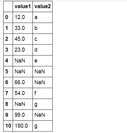
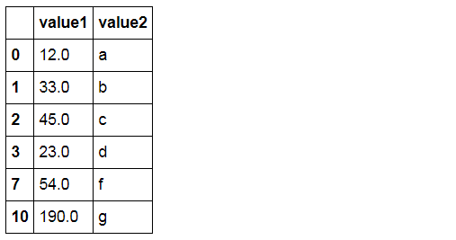
s = pd.Series([12,33,45,23,np.nan,np.nan,66,54,np.nan,99])
df = pd.DataFrame({'value1':[12,33,45,23,np.nan,np.nan,66,54,np.nan,99,190],
                  'value2':['a','b','c','d','e',np.nan,np.nan,'f','g',np.nan,'g']})
df
# 创建数据
判断是否有缺失值数据 - isnull,notnull
isnull:缺失值为True,非缺失值为False
notnull:缺失值为False,非缺失值为True
print(s.isnull()) #布尔型的一个结果,只要有一个是NaN就是True; Series直接判断是否是缺失值,返回一个Series
print(df.notnull())#判断不是缺失值的有哪些,可以加索引判断如print(df['value1'].notnull()) ;直接判断是否是缺失值,返回一个Series
0    False
1    False
2    False
3    False
4     True
5     True
6    False
7    False
8     True
9    False
dtype: bool

   value1 value2
0    True   True
1    True   True
2    True   True
3    True   True
4   False   True
5   False  False
6    True  False
7    True   True
8   False   True
9    True  False
10   True   True
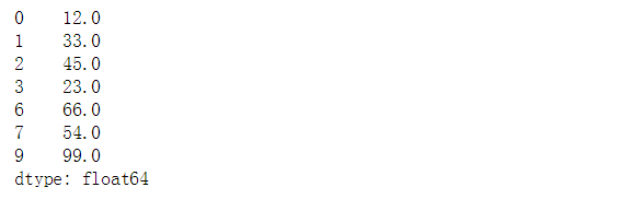
print(s[s.isnull() == False]) #把不是缺失值的给找出来。
print(df[df['value2'].notnull()])  # 注意和 df2 = df[df['value2'].notnull()] ['value1'] 的区别
##筛选非缺失值
2. 删除缺失值 - dropna
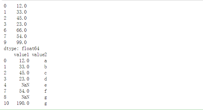
# 删除缺失值 - dropna

s = pd.Series([12,33,45,23,np.nan,np.nan,66,54,np.nan,99])
df = pd.DataFrame({'value1':[12,33,45,23,np.nan,np.nan,66,54,np.nan,99,190],
                  'value2':['a','b','c','d','e',np.nan,np.nan,'f','g',np.nan,'g']})
# 创建数据
s.dropna(inplace = True)
s
df.dropna(inplace = True)
df
3.填充/替换缺失值
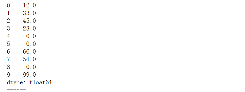
# 填充/替换缺失数据 - fillna、replace

s = pd.Series([12,33,45,23,np.nan,np.nan,66,54,np.nan,99])
df = pd.DataFrame({'value1':[12,33,45,23,np.nan,np.nan,66,54,np.nan,99,190],
                  'value2':['a','b','c','d','e',np.nan,np.nan,'f','g',np.nan,'g']})
# 创建数据
s.fillna(0,inplace = True)
print(s)
print('------')
# s.fillna(value=None, method=None, axis=None, inplace=False, limit=None, downcast=None, **kwargs)
# value:填充值
# 注意inplace参数
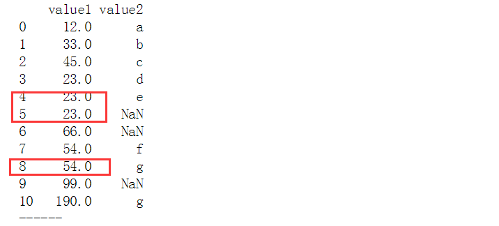
df['value1'].fillna(method = 'pad',inplace = True)
print(df)
print('------')
# method参数:
# pad / ffill → 用之前的数据填充
# backfill / bfill → 用之后的数据填充
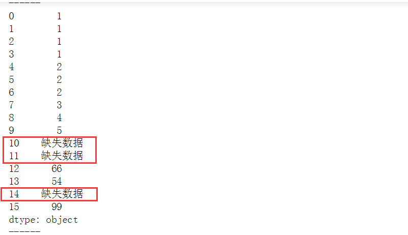
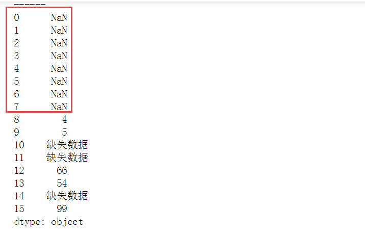
s = pd.Series([1,1,1,1,2,2,2,3,4,5,np.nan,np.nan,66,54,np.nan,99])
s.replace(np.nan,'缺失数据',inplace = True)
print(s)
print('------')
# df.replace(to_replace=None, value=None, inplace=False, limit=None, regex=False, method='pad', axis=None)
# to_replace → 被替换的值
# value → 替换值

s.replace([1,2,3],np.nan,inplace = True)
print(s)
# 多值用np.nan代替
4.缺失值插补
(1)均值/中位数/众数补插
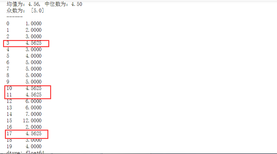
# 缺失值插补
# 几种思路:均值/中位数/众数插补、临近值插补、插值法
# (1)均值/中位数/众数插补

s = pd.Series([1,2,3,np.nan,3,4,5,5,5,5,np.nan,np.nan,6,6,7,12,2,np.nan,3,4])
#print(s)
print('------')
# 创建数据

u = s.mean()     # 均值
me = s.median()  # 中位数
mod = s.mode()   # 众数
print('均值为:%.2f, 中位数为:%.2f' % (u,me))
print('众数为:', mod.tolist())
print('------')
# 分别求出均值/中位数/众数

s.fillna(u,inplace = True)
print(s)
# 用均值填补
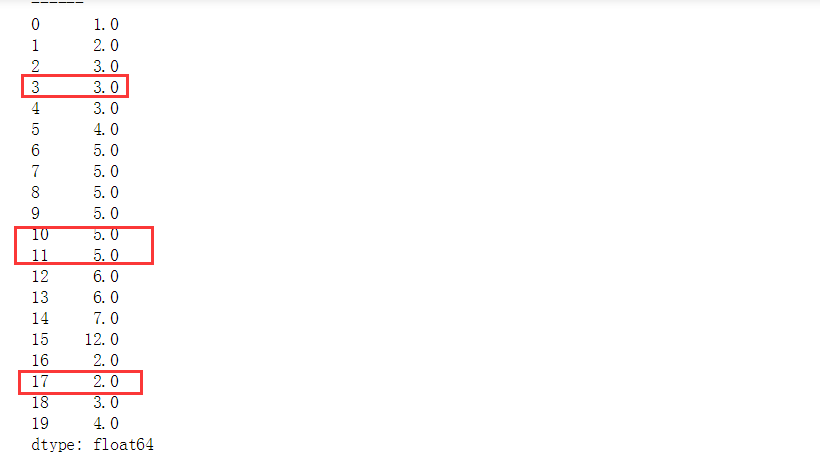
(2)临近值插补
# 缺失值插补
# 几种思路:均值/中位数/众数插补、临近值插补、插值法
# (2)临近值插补

s = pd.Series([1,2,3,np.nan,3,4,5,5,5,5,np.nan,np.nan,6,6,7,12,2,np.nan,3,4])
#print(s)
print('------')
# 创建数据

s.fillna(method = 'ffill',inplace = True)
print(s)
# 用前值插补
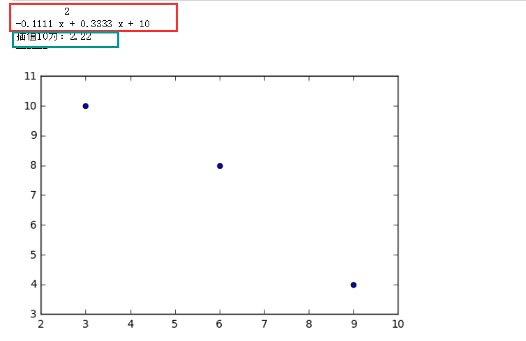
(3)插值法---拉格朗日插值法
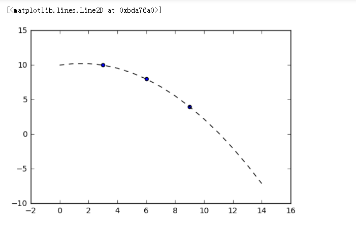
# 缺失值插补
# 几种思路:均值/中位数/众数插补、临近值插补、插值法
# (3)插值法 —— 拉格朗日插值法
from scipy.interpolate import lagrange
x = [3, 6, 9]
y = [10, 8, 4]
plt.scatter(x, y)
print(lagrange(x, y)) #直接输出多项式的方程
# 的输出值为的是多项式的n个系数
# 这里输出3个值,分别为a0,a1,a2
# y = a0 * x**2 + a1 * x + a2 → y = -0.11111111 * x**2 + 0.33333333 * x + 10

print('插值10为:%.2f' % lagrange(x,y)(10))
print('------')
# -0.11111111*100 + 0.33333333*10 + 10 = -11.11111111 + 3.33333333 +10 = 2.22222222
用少数身边的临近值去推测这个值的本身,

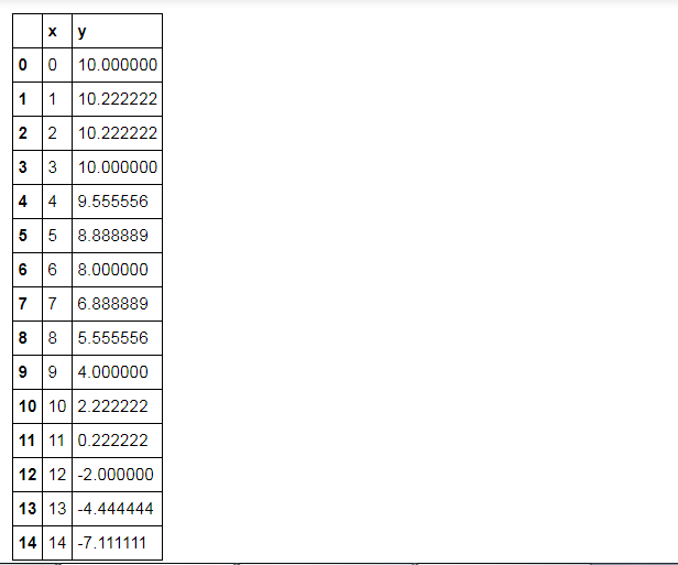
df = pd.DataFrame({'x':np.arange(15)}) #创建一个数组
df['y'] = lagrange(x, y)(df['x']) #加一个y的标签
df
plt.plot(df['x'], df['y'], linestyle = '--', color = 'k')
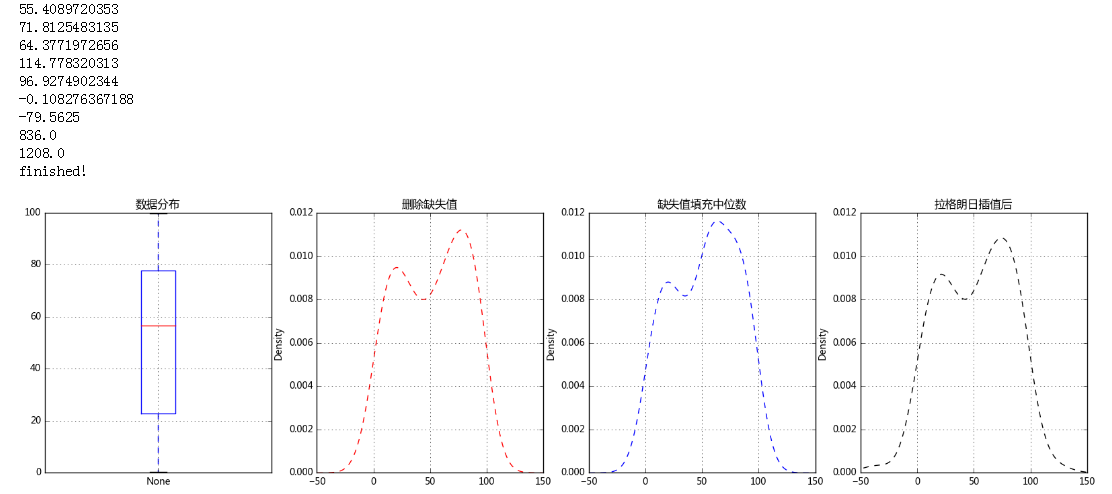
# 缺失值插补
# 几种思路:均值/中位数/众数插补、临近值插补、插值法
# (3)插值法 —— 拉格朗日插值法,实际运用

data = pd.Series(np.random.rand(100)*100)
data[3,6,33,56,45,66,67,80,90] = np.nan
print(data.head())
print('总数据量:%i' % len(data))
print('------')
# 创建数据

data_na = data[data.isnull()]
print('缺失值数据量:%i' % len(data_na))
print('缺失数据占比:%.2f%%' % (len(data_na) / len(data) * 100))
# 缺失值的数量

data_c = data.fillna(data.median())  #  中位数填充缺失值
fig,axes = plt.subplots(1,4,figsize = (20,5))
data.plot.box(ax = axes[0],grid = True,title = '数据分布')  #直接生成图,做一个密度图会直接排除缺失值。
data.plot(kind = 'kde',style = '--r',ax = axes[1],grid = True,title ='删除缺失值',xlim = [-50,150])
data_c.plot(kind = 'kde',style = '--b',ax = axes[2],grid = True,title ='缺失值填充中位数',xlim = [-50,150])
# 密度图查看缺失值情况

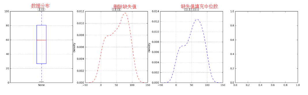
def na_c(s,n,k=5): #5为位置
    y = s[list(range(n-k,n+1+k))] # 取数
    y = y[y.notnull()]  # 剔除空值,把缺失值去掉,非缺失值筛选出来
    return(lagrange(y.index,list(y))(n))
# 创建函数,做插值,由于数据量原因,以空值前后5个数据(共10个数据)为例做插值

na_re = []
for i in range(len(data)):
    if data.isnull()[i]: #判断data里边的缺失值
        data[i] = na_c(data,i)
        print(na_c(data,i))
        na_re.append(data[i])
data.dropna(inplace=True)  # 清除插值后仍存在的缺失值
data.plot(kind = 'kde',style = '--k',ax = axes[3],grid = True,title = '拉格朗日插值后',xlim = [-50,150])
print('finished!')
# 缺失值插值