暑期学习 GAN 笔记
前言:
GAN 是 对抗生成网络 (Generative Adversarial Networks)。2014年还在蒙特利尔读博的 Ian Goodfellow 将 GAN 引入到 DL 领域。去年,也就是2016年,是 GAN 最火的一年,大量论文被发表,今年淡了一些。
- 下图(把马变成斑马,就是GAN的一种应用)

一、GAN 原理概述
简单说, GAN 的工作,就是找出某种对象事物的特征,并且能够基于所学到的特征,计算机自主产生一个新的这类事物对象。这是一个从无到有的过程。
举例,GAN 学习1-9个数字的形状特征,计算机基于学习的特征自动生成新的数字形状。
二、趣说 GAN 原理
GAN 包括两个主要模块:
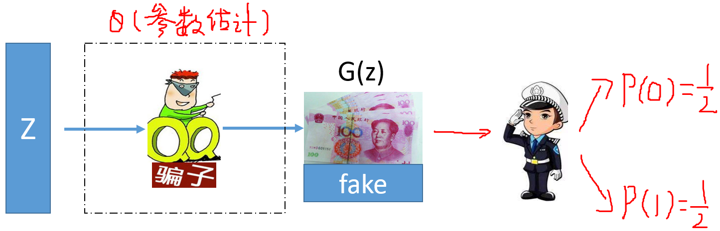
- 生成器 (骗子)
- 判别器 (警察)
GAN ------ 骗子和警察的故事。
1、生成器 G(骗子)
-
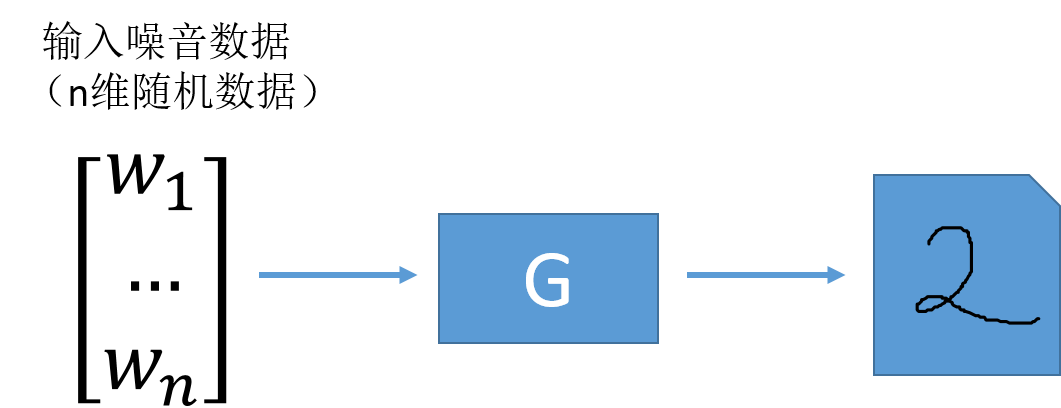
G 的作用:将噪音数据产生为逼近真实的数据。
-
以数字灰度图像为例;G 需要有输入 ,输入往往是噪音随机数据的向量;输入经过 G 生成的便是仿真的数字图像。
-
G 前面是一个 输入层。
2、判别器 D(警察)
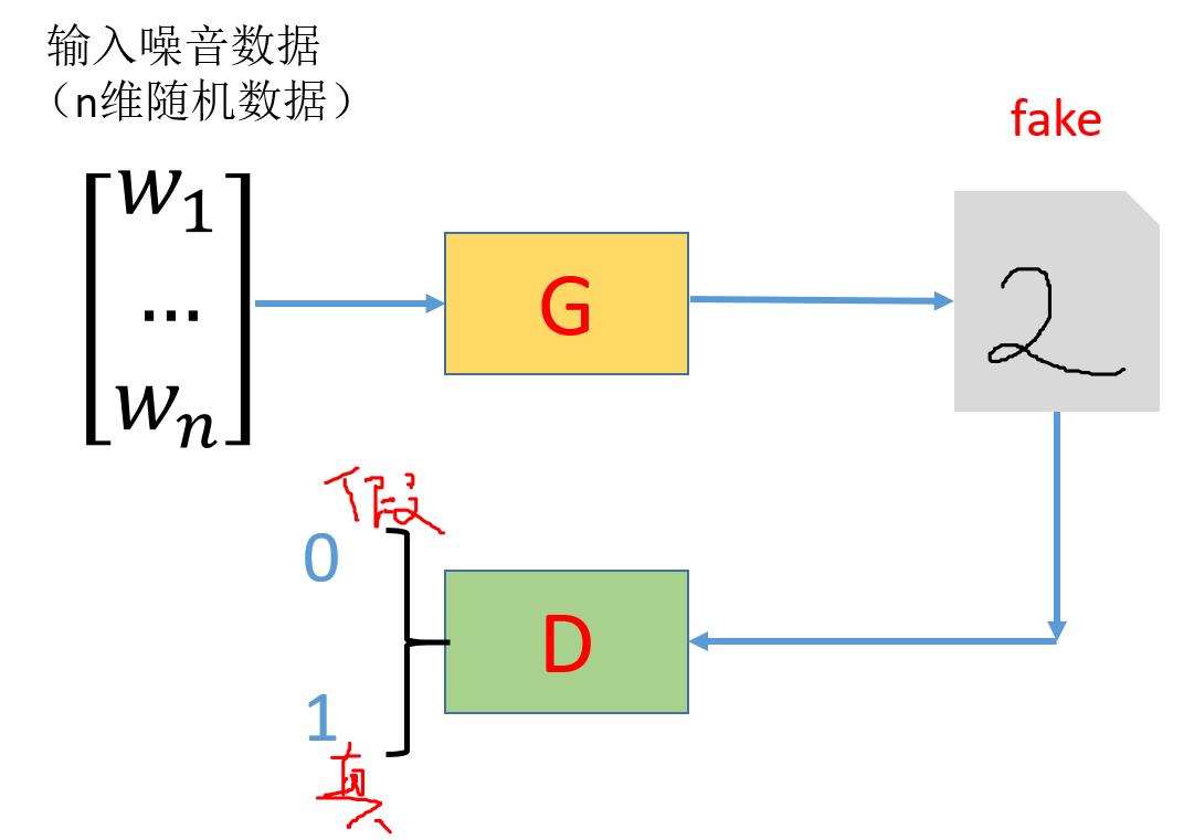
- D 的作用:将 G 生产的仿真数据判断是真是假,实际上为一个二分类器。
- 一个有趣的比喻:

我们希望网络可以做到:
1 --------- G 生成的仿真数据越真越好 骗过 D;(以假乱真)
2 --------- D 能够分辨出仿真数据是假的 [real →1、fake → 0];(真假分明)1 --------- 骗子 G 仿造的纸币能够 以假乱真 骗过警察;
2 --------- 警察 D 能够辨别出骗子制造的假货以及能够识别出真货,分辨能力越强越好;
因此,GAN 中同时优化 G 和 D 两种网络:(类似于 周伯通的左右手互搏)
生成器:瞒天过海
判别器:火眼金睛
损失函数定义 : 一方面要让判别器分辨能力更强,另一方面要让生成器更真 。
最后达到的效果是:生成器生成的 fake 太逼近真实而让判别器不能分辨。

3、细说D、G网络
网络的工作目的:
噪音数据经过 G 网络的参数估计求出一组参数值 ;通过参数的作用将噪音数据变换为新样本。
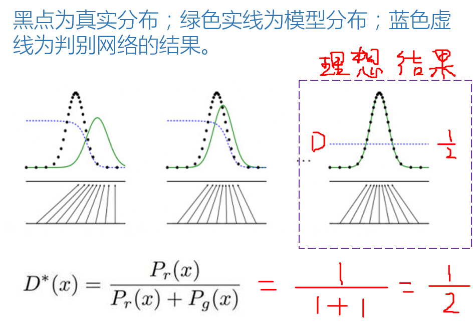
最终的想法是达到 G 网络在分辨能力很强的基础上,都无法判别新样本是真是假;结果是新样本输入到 D 得到的为真 和 为假 的 概率各占一半。最后 D 无法分辨生成的图片和真实图片,GAN 网络就拟合了。
网络的工作方式:
生成器是一种寻找分布最优参数的过程,而这些参数的更新不是来自于数据样本本身(不是对数据的似然性进行优化),而是来自于判别器 D 的一个反传梯度。
-
问题:G 和 D 是如何联合工作去拟合一个很好的分布 g ,( 是这个分布的参数,如高斯分布中 就是每个高斯分布的期望和方差),具体过程参考如下文章。
D 网络策略:
黑点:真实 Data 的分布 r
绿色实线:生成 Model 的分布 g
* :应该是两个分布之间的占比值
三、GAN 网络结构
前言: 本例以 MNIST 数据集做示范。
1、导入库
import tensorflow as tf
import numpy as np
# ```pickle库可以将结果保存到本地```
import pickle
import matplotlib.pyplot as plt

%matplotlib inline
- 导入MNIST数据
###2、网络架构###
输入层 :待生成图像(噪音数据)和真实数据
生成网络:将噪音图像进行生成
判别网络:
- (1)判断真实图像输出结果
- (2)判断生成图像输出结果
目标函数:
- (1)对于生成网络要 使得生成结果通过判别网络为真
- (2)对于判别网络要使得 输入为真实图像时判别为真;输入为生成图像时判别为假
- 好好理解这个 目标函数:
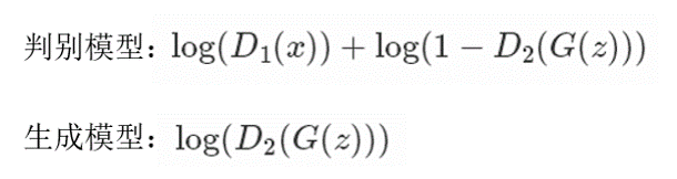
解读 生成模型 目标函数:
:是输入到生成器产生的结果。
:是通过判别网络的结果;(在该函数中为 2)。
:增函数意味着自变量越大,函数值越大;我们希望生成器的效果令 判别其为真(真为1),则 越接近于1, 越接近于0。
解读 判别模型 目标函数:
注意:判别模型有 两种 输入,即 、 ;两者共享一组权重参数,本质上 、 是同一个网络,输入不同。
:对应真实数据通过判别网络的结果;( 对应噪音生成数据通过判别网络的结果)。
:我们希望判别器的效果令 能够火眼金睛识真(真为1),则 越接近于1, 越接近于0;同理可知,我们也同时希望判别器的效果令 能够火眼金睛辨假(假为0),则 接近于1, 接近于0。
3、输入层
- 输入层输入两种数据:
- 噪音数据
- 真实数据
#真实数据和噪音数据
def get_inputs(real_size, noise_size):
    # placeholder 类似于占位符
    #真实图像的tensor和噪音图像的tensor
    real_img = tf.placeholder(tf.float32, [None, real_size])
    noise_img = tf.placeholder(tf.float32, [None, noise_size])

    return real_img, noise_img
4、定义生成器
- 生成器
- noise_img: 产生的噪音输入
- n_units: 隐层单元(神经元)个数
- out_dim: 输出的大小(28 * 28 * 1)
关于 leaky-ReLu:
[1] 近年来,ReLU 变的越来越受欢迎。它的数学表达式如下:
[2] leaky ReLU 是用来解决 “dying ReLU” 问题的。与 ReLU 不同的是:
这里的 α 是一个很小的常数。 这样,既修正了数据分布,又保留了部分负轴的值,使得负轴信息不会全部丢失。
当 时, ;
当 时, ;
公式表达为 ,或者可以表达为 ;
由于 是一个很小的正数,当 时, 一定比 大,在该条件下结果取 ;
当 时, 一定比 大,该条件下结果取 。对应代码即:
tf.maximum(layer*alpha, layer)
def get_generator(noise_img, n_units, out_dim, reuse=False, alpha=0.01):
# reuse 参数要不要重新利用(D1\D2);G不需要故reuse=False
# scope_generator_变量域
with tf.variable_scope("generator", reuse=reuse):
# hidden layer
hidden1 = tf.layers.dense(noise_img, n_units)
# leaky ReLU
hidden1 = tf.maximum(alpha * hidden1, hidden1)
# dropout
hidden1 = tf.layers.dropout(hidden1, rate=0.2)
# logits 得分值 & outputs
# 神经网络的最后一层是逻辑层,这层会返回我们的预测原始结果值
# out_dim 是生成器的输出tensor的size。
logits = tf.layers.dense(hidden1, out_dim)
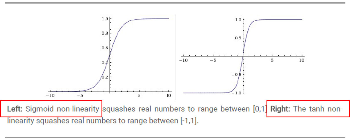
# 压缩到(-1,1)
outputs = tf.tanh(logits)
return logits, outputs
- sigmoid VS tanh ( 双曲正切 )
5、定义判别器
- 判别器
- img:输入
- n_units:隐层单元数量
- reuse:由于要使用两次
def get_discriminator(img, n_units, reuse=False, alpha=0.01):
    # scope_discriminator_变量域
    with tf.variable_scope("discriminator", reuse=reuse):
        # hidden layer
        hidden1 = tf.layers.dense(img, n_units)
        hidden1 = tf.maximum(alpha * hidden1, hidden1)

        # logits & outputs
        logits = tf.layers.dense(hidden1, 1)
        outputs = tf.sigmoid(logits)

        return logits, outputs
6、设置网络参数、构建网络
- 网络参数定义
- img_size:输入大小
- noise_size:噪音图像大小
- g_units:生成器隐层参数
- d_units:判别器隐层参数
- learning_rate:学习率
img_size = mnist.train.images[0].shape[0]

noise_size = 100

g_units = 128

d_units = 128

learning_rate = 0.001

alpha = 0.01
tf.reset_default_graph()

real_img, noise_img = get_inputs(img_size, noise_size)

# generator
g_logits, g_outputs = get_generator(noise_img, g_units, img_size)

# discriminator
d_logits_real, d_outputs_real = get_discriminator(real_img, d_units)
d_logits_fake, d_outputs_fake = get_discriminator(g_outputs, d_units, reuse=True) # reuse=True
四、训练网络
1、实现目标函数
# discriminator的loss
# 识别真实图片(d_logits_real预测值和tf.ones_like真实值之间的差)
d_loss_real = tf.reduce_mean(tf.nn.sigmoid_cross_entropy_with_logits(logits=d_logits_real,
                                                                     labels=tf.ones_like(d_logits_real)))
# 识别生成的图片(d_logits_fake预测值和tf.zeros_like真实值之间的差)
d_loss_fake = tf.reduce_mean(tf.nn.sigmoid_cross_entropy_with_logits(logits=d_logits_fake,
                                                                     labels=tf.zeros_like(d_logits_fake)))
# 总体loss
d_loss = tf.add(d_loss_real, d_loss_fake)
#=====================================#
# generator的loss(d_logits_fake预测值和tf.ones_like真实值之间的差,以假乱真)
g_loss = tf.reduce_mean(tf.nn.sigmoid_cross_entropy_with_logits(logits=d_logits_fake,
                                                                labels=tf.ones_like(d_logits_fake)))
2、优化器
注:下面定义了优化函数,由于 GAN 中包含了生成器和判别器两种网络,因此优化需要分开进行;所以在这块之前定义 variable_scope 的原因就是如此。
train_vars = tf.trainable_variables()

# generator中的tensor
g_vars = [var for var in train_vars if var.name.startswith("generator")] # "generator"域下变量
# discriminator中的tensor
d_vars = [var for var in train_vars if var.name.startswith("discriminator")] # "discriminator"域下变量

# optimizer/AdamOptimizer自动调整学习率
d_train_opt = tf.train.AdamOptimizer(learning_rate).minimize(d_loss, var_list=d_vars)
g_train_opt = tf.train.AdamOptimizer(learning_rate).minimize(g_loss, var_list=g_vars)
3、训练
# batch_size
batch_size = 64
# 训练迭代轮数
epochs = 300
# 抽取样本数
n_sample = 25

# 存储测试样例
samples = []
# 存储loss
losses = []
# 保存生成器变量
saver = tf.train.Saver(var_list = g_vars)
# 开始训练
with tf.Session() as sess:
    sess.run(tf.global_variables_initializer())
    for e in range(epochs):
        for batch_i in range(mnist.train.num_examples//batch_size):
            batch = mnist.train.next_batch(batch_size)

            batch_images = batch[0].reshape((batch_size, 784))
            # 对图像像素进行scale,这是因为tanh输出的结果介于(-1,1),real和fake图片共享discriminator的参数
            batch_images = batch_images*2 - 1

            # generator的输入噪声
            batch_noise = np.random.uniform(-1, 1, size=(batch_size, noise_size))

            # Run optimizers
            _ = sess.run(d_train_opt, feed_dict={real_img: batch_images, noise_img: batch_noise})
            _ = sess.run(g_train_opt, feed_dict={noise_img: batch_noise})

        # 每一轮结束计算loss
        train_loss_d = sess.run(d_loss,
                                feed_dict = {real_img: batch_images,
                                             noise_img: batch_noise})
        # real img loss
        train_loss_d_real = sess.run(d_loss_real,
                                     feed_dict = {real_img: batch_images,
                                                 noise_img: batch_noise})
        # fake img loss
        train_loss_d_fake = sess.run(d_loss_fake,
                                    feed_dict = {real_img: batch_images,
                                                 noise_img: batch_noise})
        # generator loss
        train_loss_g = sess.run(g_loss,
                                feed_dict = {noise_img: batch_noise})


        print("Epoch {}/{}...".format(e+1, epochs),
              "判别器损失: {:.4f}(判别真实的: {:.4f} + 判别生成的: {:.4f})...".format(train_loss_d, train_loss_d_real, train_loss_d_fake),
              "生成器损失: {:.4f}".format(train_loss_g))

        losses.append((train_loss_d, train_loss_d_real, train_loss_d_fake, train_loss_g))

        # 保存样本
        sample_noise = np.random.uniform(-1, 1, size=(n_sample, noise_size))
        gen_samples = sess.run(get_generator(noise_img, g_units, img_size, reuse=True),
                               feed_dict={noise_img: sample_noise})
        samples.append(gen_samples)


        saver.save(sess, './checkpoints/generator.ckpt')

# 保存到本地
with open('train_samples.pkl', 'wb') as f:
    pickle.dump(samples, f)
4、生成结果
- loss迭代曲线
fig, ax = plt.subplots(figsize=(20,7))
losses = np.array(losses)
plt.plot(losses.T[0], label='判别器总损失')
plt.plot(losses.T[1], label='判别真实损失')
plt.plot(losses.T[2], label='判别生成损失')
plt.plot(losses.T[3], label='生成器损失')
plt.title("对抗生成网络")
ax.set_xlabel('epoch')
plt.legend()
- 查看生成结果
# Load samples from generator taken while training
with open('train_samples.pkl', 'rb') as f:
    samples = pickle.load(f)

#samples是保存的结果 epoch是第多少次迭代
def view_samples(epoch, samples):

    fig, axes = plt.subplots(figsize=(7,7), nrows=5, ncols=5, sharey=True, sharex=True)
    for ax, img in zip(axes.flatten(), samples[epoch][1]): # 这里samples[epoch][1]代表生成的图像结果,而[0]代表对应的logits
        ax.xaxis.set_visible(False)
        ax.yaxis.set_visible(False)
        im = ax.imshow(img.reshape((28,28)), cmap='Greys_r')

    return fig, axes

#查看指定最终的结果
_ = view_samples(-1, samples) # 显示最终的生成结果
# 指定要查看的轮次
epoch_idx = [10, 30, 60, 90, 120, 150, 180, 210, 240, 290]
show_imgs = []
for i in epoch_idx:
    show_imgs.append(samples[i][1])
# 指定图片形状
rows, cols = 10, 25
fig, axes = plt.subplots(figsize=(30,12), nrows=rows, ncols=cols, sharex=True, sharey=True)

idx = range(0, epochs, int(epochs/rows))

for sample, ax_row in zip(show_imgs, axes):
    for img, ax in zip(sample[::int(len(sample)/cols)], ax_row):
        ax.imshow(img.reshape((28,28)), cmap='Greys_r')
        ax.xaxis.set_visible(False)
        ax.yaxis.set_visible(False)
# 加载我们的生成器变量
saver = tf.train.Saver(var_list=g_vars)
with tf.Session() as sess:
    saver.restore(sess, tf.train.latest_checkpoint('checkpoints'))
    # 噪声数据生成25个样本
    sample_noise = np.random.uniform(-1, 1, size=(25, noise_size))
    gen_samples = sess.run(get_generator(noise_img, g_units, img_size, reuse=True),
                           feed_dict={noise_img: sample_noise})
_ = view_samples(0, [gen_samples])