传统算法(一):
线性回归
一、什么是线性回归
线性回归是利用数理统计中回归分析,来确定两种或两种以上变量间相互依赖的定量关系的一种统计分析方法,运用十分广泛。
举一个栗子数据:
工资和年龄(2个特征)
目标:预测银行会贷款给我多少钱(标签)
线性回归考虑:工资和年龄都会影响最终银行贷款的结果那么它们各自有多大的影响呢?(参数)
| 工资 | 年龄 | 额度 |
|---|---|---|
| 4000 | 25 | 12000 |
| 8000 | 28 | 15000 |
| 12000 | 35 | 20000 |
| 15000 | 40 | 25000 |
所以,通俗的解释就是:
x1,x2对应的就是工资和年龄两个变量,而y就是最终银行会批的额度;线性回归就是建立关于X与Y的一个方程式;
二、建立目标函数
接下来根据上面的例子,我们来建立目标函数
假设 是年龄参数, 是工资参数
拟合的平面则为:
整合,可得如下:
当然真实值和预测值之间肯定是要存在差异的,这个称作“误差”
误差项:
公式中我们
用来表示该误差值,那可以进一步得到目标函数为:
这里每一个
都会对应有
,并且假设
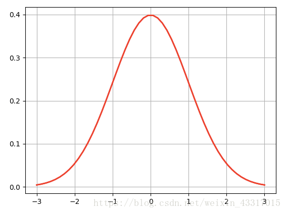
均值为0,方差为
,且服从高斯分布,也就是正态分布。
那么我们可以知道
概率为:
将目标函数转换为: 并带入以上公式,可得:
我们的目标当然是要误差项越小越好,这个时候我们要借用似然函数来让我们找到最好的参数值,让目标预测值越接近真实值。
三、引入似然函数
似然函数是对函数进行累乘,用样本估计参数值,故我们希望似然函数越大越好,最后得到的是真实值的概率。
似然函数要求最大值,我们通过对数的性质,将累乘转换为累加,转为对数似然:
转换为累加:
因为我们需要似然函数越大越好,所以对于上式,就希望
值越小越好,而这个式子,就是常说的最小二乘法,也是损失函数。
转换为:
通过求偏导来求得最小值:
令
,可以得出
的表达式:
四、梯度下降
梯度下降算法的思想通俗的解释可以为:假设我们站在山顶,我们需要选择最快最优的方法从山顶下到最低点;
接下来的做法是:
- 首先是随机选择一个站的位置(参数的组合),然后对这个点进行最小值的计算;
- 然后是不断改变,并计算代价函数,直到一个局部最小值。之所以是局部最小值,是因为我们并没有尝试完所有的参数组合,所以不能确定我们得到的局部最小值是否便是全局最小值;
- 最后尝试选择不同的初始参数组合,可能会找到不同的局部最小值。
因为我们的损失函数是:
将目标函数
带入损失函数,并进行求偏导:
这里我们介绍3种不同的梯度下降的方法,可以针对不同的情况,来选择不同的方法,同时会增加一个 值,表示的是学习率(learning rate) ,它决定了我们沿着能让代价函数下降程度最大的方向向下迈进的步子有多大:
- 批量梯度下降(batch gradient descent):计算的是所有样本量;
优点:因为是对所有样本计算,所以容易得到最优解;
缺点:如果样本量较大,这样计算的速度会狠慢;
批量梯度下降算法的公式为:
- 随机梯度下降(random gradient descent):每次都随机找一个样本计算;
优点:计算迭代的速度比较快;
缺点:不一定每次都朝着收敛的方向;
随机梯度下降算法的公式为:
- 小批量梯度下降(small batch gradient descent):每次选择一部分计算;
优点:实用性较高,计算较快;
缺点:不一定最后算的是全局的最小值;
小批量梯度下降算法的公式为:
这样我们通过最小二乘法以及梯度下降的方式,都求出了 的最优参数,使得误差最小;
五、Python代码实现
使用sklearn模块中的线性回归算法的代码:
import numpy as np
import pandas as pd
from sklearn import linear_model
import matplotlib.pyplot as plt
from sklearn.model_selection import cross_val_predict,KFold,train_test_split
from sklearn.linear_model import LinearRegression
#传入需要进行预测的数据
loans = pd.read_csv('./data/cleaned_loans2007.csv')
#实例化算法
lr = LinearRegression(class_weight='balanced')
train,test = train_test_split(loans,test_size=0.3)
#对模型进行训练
lr.fit(train.loc[:,train.columns !='loan_status'],train['loan_status'])
#输出预测值
predict = lr.predict(train.loc[:,train.columns !='loan_status'])
predict = pd.Series(predict)
#通过False positive rate(FPR)以及True positive rate(TPR)进行判断模型是否可行
fp = (predict==0)& (train['loan_status'] ==1)
tp = (predict==0)& (train['loan_status'] ==0)
fn = (predict==1)& (train['loan_status'] ==0)
tn = (predict==1)& (train['loan_status'] ==1)

FPR = fp.sum()/(fp.sum()+tn.sum())
TPR = tp.sum()/(tp.sum()+fn.sum())
print(FPR,TPR)
不使用已有算法方法,来写线性回归算法的代码:
以下代码参考Part 1 - Simple Linear Regression
import os
import numpy as np
import pandas as pd
import matplotlib.pylab as plt
from sklearn import linear_model

# 计算损失函数
def computeCost(X, y, theta):
    inner = np.power(((X * theta.T) - y), 2)
    return np.sum(inner) / (2 * len(X))

# 梯度下降算法
def gradientDescent(X, y, theta, alpha, iters):
    temp = np.matrix(np.zeros(theta.shape))
    parameters = int(theta.ravel().shape[1])
    cost = np.zeros(iters)

    for i in range(iters):
        error = (X * theta.T) - y

        for j in range(parameters):
            # 计算误差对权值的偏导数
            term = np.multiply(error, X[:, j])
            # 更新权值
            temp[0, j] = theta[0, j] - ((alpha / len(X)) * np.sum(term))

        theta = temp
        cost[i] = computeCost(X, y, theta)
    return theta, cost

dataPath = os.path.join('data', 'ex1data1.txt')
data = pd.read_csv(dataPath, header=None, names=['Population', 'Profit'])
# print(data.head())
# print(data.describe())
# data.plot(kind='scatter', x='Population', y='Profit', figsize=(12, 8))
# 在数据起始位置添加1列数值为1的数据
data.insert(0, 'Ones', 1)
print(data.shape)

cols = data.shape[1]
X = data.iloc[:, 0:cols-1]
y = data.iloc[:, cols-1:cols]

# 从数据帧转换成numpy的矩阵格式
X = np.matrix(X.values)
y = np.matrix(y.values)
# theta = np.matrix(np.array([0, 0]))
theta = np.matrix(np.zeros((1, cols-1)))
print(theta)
print(X.shape, theta.shape, y.shape)
cost = computeCost(X, y, theta)
print("cost = ", cost)

# 初始化学习率和迭代次数
alpha = 0.01
iters = 1000

# 执行梯度下降算法
g, cost = gradientDescent(X, y, theta, alpha, iters)
print(g)

# 可视化结果
x = np.linspace(data.Population.min(),data.Population.max(),100)
f = g[0, 0] + (g[0, 1] * x)

fig, ax = plt.subplots(figsize=(12, 8))
ax.plot(x, f, 'r', label='Prediction')
ax.scatter(data.Population, data.Profit, label='Training Data')
ax.legend(loc=2)
ax.set_xlabel('Population')
ax.set_ylabel('Profit')
ax.set_title('Predicted Profit vs. Population Size')

fig, ax = plt.subplots(figsize=(12, 8))
ax.plot(np.arange(iters), cost, 'r')
ax.set_xlabel('Iteration')
ax.set_ylabel('Cost')
ax.set_title('Error vs. Training Epoch')
以上,就是本次学习的线性回归的数学推导,以及python代码实现的案例;