tensorflow 10： sofmax回归识别mnist手写数字图片

版权声明：本文为博主原创文章，转载请标明原始博文地址。 https://blog.csdn.net/yuanlulu/article/details/82944700

Softmax回归介绍

为了得到一张给定图片属于某个特定数字类的证据（evidence），我们对图片像素值进行加权求和。如果这个像素具有很强的证据说明这张图片不属于该类，那么相应的权值为负数，相反如果这个像素拥有有利的证据支持这张图片属于这个类，那么权值是正数。我们也需要加入一个额外的偏置量（bias），因为输入往往会带有一些无关的干扰量。

下面的图片显示了一个模型学习到的图片上每个像素对于特定数字类的权值。红色代表负数权值，蓝色代表正数权值。

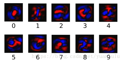
可以看到，基本每个数字的权重就是该数字外形的模板。

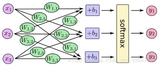
对于softmax回归模型可以用下面的图解释，对于输入的xs加权求和，再分别加上一个偏置量，最后再输入到softmax函数中：

我们也可以用向量表示这个计算过程：用矩阵乘法和向量相加。这有助于提高计算效率。（也是一种更有效的思考方式）

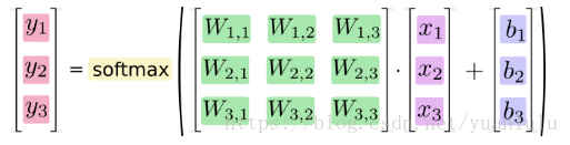
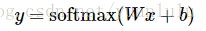
更进一步，可以写成更加紧凑的方式：

代码范例1

原理分步讲解

本节代码参考《TensorFlow实现SoftMax Regression分类器》，文字修改自《MNIST机器学习入门》，其实就是tensorflow官方教程的中文版。

0. Input: 定义输入节点

X = tf.placeholder(tf.float32, shape=[None, 784], name='X')
Y_true = tf.placeholder(tf.float32, shape=[None, 10], name='Y_true')

X不是一个特定的值，而是一个占位符placeholder，我们在TensorFlow运行计算时输入这个值。我们希望能够输入任意数量的MNIST图像，每一张图展平成784维的向量。我们用2维的浮点数张量来表示这些图，这个张量的形状是[None，784 ]。（这里的None表示此张量的第一个维度可以是任何长度的。）

Y_true采用的是一种叫做独热编码的形式来表示。

1. Inference:前向预测

W = tf.Variable(tf.zeros([784, 10]), name="Weight")
b = tf.Variable(tf.zeros([10]), name="Bias")
logits = tf.add(tf.matmul(X, W), b)

# softmax把logits变成预测概率分布
Y_pred = tf.nn.softmax( logits=logits )

注意，W的维度是[784，10]，因为我们想要用784维的图片向量乘以它以得到一个10维的证据值向量，每一位对应不同数字类。b的形状是[10]，所以我们可以直接把它加到输出上面。

Y_pred的形状是[? ,10],其中?是每个batch的大小。

2. Loss:定义损失节点

这里的损失使用的是交叉熵。
它的形式为：

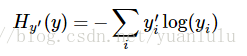
y 是我们预测的概率分布, y’ 是实际的分布（我们输入的one-hot vector)。比较粗糙的理解是，交叉熵是用来衡量我们的预测用于描述真相的低效性。

由于训练的时候是每次训练一批（下面的代码中batch size是100）,所以Y_pred和Y_true的形状是[100, 10],还要把所有的图片的交叉熵求和之后求平均。

TrainLoss = tf.reduce_mean(-tf.reduce_sum(Y_true * tf.log(Y_pred), axis=1))

3. Train:定义训练节点

现在TensorFlow拥有一张描述你各个计算单元的图，它可以自动地使用反向传播算法(backpropagation algorithm)来有效地确定你的变量是如何影响你想要最小化的那个成本值的。然后，TensorFlow会用你选择的优化算法来不断地修改变量以降低成本。

# Optimizer: 创建一个梯度下降优化器
Optimizer = tf.train.GradientDescentOptimizer(learning_rate=0.01)
# Train: 定义训练节点将梯度下降法应用于Loss
TrainStep = Optimizer.minimize(TrainLoss)

在这里，我们要求TensorFlow用梯度下降算法（gradient descent algorithm）以0.01的学习速率最小化交叉熵。梯度下降算法（gradient descent algorithm）是一个简单的学习过程，TensorFlow只需将每个变量一点点地往使成本不断降低的方向移动。

4. Evaluate: 定义评估节点

correct_prediction = tf.equal(tf.argmax(Y_pred, 1), tf.argmax(Y_true, 1))
accuracy = tf.reduce_mean(tf.cast(correct_prediction, tf.float32))

Y_true是独热编码，除了1个为1的成员其它为0。Y_pred是类似的，只是每个成员都是小于1的浮点数，总和为1.
只要求两者最大值的下标是否相等，即可知道是否预测正确。
correct_prediction会给我们一组布尔值。为了确定正确预测项的比例，我们可以把布尔值转换成浮点数，然后取平均值，得到最终的准确率。correct_prediction的形状是[bathc_size],在下面的代码中等于100.

代码

本节代码参考《TensorFlow实现SoftMax Regression分类器》，我在原来代码基础上做了一些调整。
除了上面的分步讲解的内容，还有为了tensirboard可视化增加的代码。
这份代码比tensorflow官网代码好在把 Inference、Loss、Train、 Evaluate单独拎开，模块化做的比较好。实际上大部分模型都可以分为这4个部分来单独编写。

代码我简单修改了一点，把Y_pred放到Inference下了，其它基本没变。

经过测试，训练的步数和准确率的关系如下。由此可见，0.92基本是这种算法的上限了。

训练次数	学习率	准确率
1000	0.01	0.87
5000	0.01	0.90
10000	0.01	0.90
1000	0.5	0.919
5000	0.5	0.92
5000	0.1	0.92

import os
import sys
import argparse
import tensorflow as tf
from tensorflow.examples.tutorials.mnist import input_data
os.environ['TF_CPP_MIN_LOG_LEVEL'] = '2'

#在main()主函数中组织整个计算图并运行会话
def main(_):
    print('~~~~~~~~~~开始设计计算图~~~~~~~~')
    # 告诉TensorFlow模型将会被构建在默认的Graph上.
    with tf.Graph().as_default():
        # Input: 定义输入节点
        with tf.name_scope('Input'):
            # 计算图输入占位符
            X = tf.placeholder(tf.float32, shape=[None, 784], name='X')
            Y_true = tf.placeholder(tf.float32, shape=[None, 10], name='Y_true')
        # Inference:前向预测,创建一个线性模型：y = x*w + b
        with tf.name_scope('Inference'):
            W = tf.Variable(tf.zeros([784, 10]), name="Weight")
            b = tf.Variable(tf.zeros([10]), name="Bias")
            logits = tf.add(tf.matmul(X, W), b)

            # softmax把logits变成预测概率分布
            with tf.name_scope( 'Softmax' ):
                Y_pred = tf.nn.softmax( logits=logits )
        # Loss:定义损失节点
        with tf.name_scope('Loss'):

            # #计算交叉熵损失
            # with tf.name_scope('CrossEntropy'):
            TrainLoss = tf.reduce_mean(
                    -tf.reduce_sum(Y_true * tf.log(Y_pred), axis=1))
        # Train:定义训练节点
        with tf.name_scope('Train'):
            # Optimizer: 创建一个梯度下降优化器
            Optimizer = tf.train.GradientDescentOptimizer(learning_rate=0.01)
            # Train: 定义训练节点将梯度下降法应用于Loss
            TrainStep = Optimizer.minimize(TrainLoss)
        #Evaluate: 定义评估节点
        with tf.name_scope('Evaluate'):
            correct_prediction = tf.equal(tf.argmax(Y_pred, 1), tf.argmax(Y_true, 1))
            accuracy = tf.reduce_mean(tf.cast(correct_prediction, tf.float32))

        # Initial:添加所有Variable类型的变量的初始化节点
        InitOp = tf.global_variables_initializer()

        print('把计算图写入事件文件，在TensorBoard里面查看')
        writer = tf.summary.FileWriter(logdir='logs/mnist_softmax', graph=tf.get_default_graph())
        writer.close()

        print('~~~~~~~~~~开始运行计算图~~~~~~~~')
        # 加载数据
        mnist = input_data.read_data_sets(FLAGS.data_dir, one_hot=True)

        # 声明一个交互式会话
        sess = tf.InteractiveSession()
        # 初始化所有变量: W、b
        sess.run(InitOp)

        # 开始按批次训练，总共训练1000个批次，每个批次100个样本
        for step in range(1000):
            batch_xs, batch_ys = mnist.train.next_batch(100)
            # 将当前批次的样本喂(feed)给计算图中的输入占位符，启动训练节点开启训练
            _, train_loss = sess.run([TrainStep, TrainLoss],
                                     feed_dict={X: batch_xs, Y_true: batch_ys})
            print("train step: ", step, ", train_loss: ", train_loss)

        accuracy_score = sess.run(accuracy,feed_dict={X: mnist.test.images,
                                                        Y_true: mnist.test.labels})
        print("模型准确率：", accuracy_score)

#调用main()函数
if __name__ == '__main__':
  #首先申明一个参数解析器对象
  parser = argparse.ArgumentParser()
  #为参数解析器添加参数：data_dir(指定数据集存放路径)
  parser.add_argument('--data_dir', type=str,
                      default='./data/',  #参数默认值
                      help='数据集存放路径')
  FLAGS, unparsed = parser.parse_known_args() #解析参数
  #运行TensorFlow应用
  tf.app.run(main=main, argv=[sys.argv[0]] + unparsed)

代码范例2

本小节的代码功能和上面基本一致。
这段代码来自tensorflow源码下的例子，目录是：tensorflow/examples/tutorials/mnist/mnist_softmax.py

下面讲讲本节代码和上一节的区别。

区别1

本节的代码没有为tensorboard提供额外信息，也没有把程序分为Inference、Loss、Train、 Evaluate几块，而是写在一个函数里面。

区别2

本节代码在做完Wx+b的计算后没有分开计算softmax和loss，而是把这两步合一，用sparse_softmax_cross_entropy来计算loss。

区别3

上节代码读取时选择独热编码的形式来返回y，本节代码没有采用独热编码。所以计算准确率的代码稍有区别。

代码

本节代码运行1000次以后在测试集上的准确率为0.91，与上一节基本相当。

# Copyright 2015 The TensorFlow Authors. All Rights Reserved.
#
# Licensed under the Apache License, Version 2.0 (the "License");
# you may not use this file except in compliance with the License.
# You may obtain a copy of the License at
#
#     http://www.apache.org/licenses/LICENSE-2.0
#
# Unless required by applicable law or agreed to in writing, software
# distributed under the License is distributed on an "AS IS" BASIS,
# WITHOUT WARRANTIES OR CONDITIONS OF ANY KIND, either express or implied.
# See the License for the specific language governing permissions and
# limitations under the License.
# ==============================================================================
"""A very simple MNIST classifier.

See extensive documentation at
https://www.tensorflow.org/get_started/mnist/beginners
"""
from __future__ import absolute_import
from __future__ import division
from __future__ import print_function

import argparse
import sys

from tensorflow.examples.tutorials.mnist import input_data

import tensorflow as tf

FLAGS = None


def main(_):
  # Import data
  mnist = input_data.read_data_sets(FLAGS.data_dir)

  # Create the model
  x = tf.placeholder(tf.float32, [None, 784])
  W = tf.Variable(tf.zeros([784, 10]))
  b = tf.Variable(tf.zeros([10]))
  y = tf.matmul(x, W) + b

  # Define loss and optimizer
  y_ = tf.placeholder(tf.int64, [None])

  # The raw formulation of cross-entropy,
  #
  #   tf.reduce_mean(-tf.reduce_sum(y_ * tf.log(tf.nn.softmax(y)),
  #                                 reduction_indices=[1]))
  #
  # can be numerically unstable.
  #
  # So here we use tf.losses.sparse_softmax_cross_entropy on the raw
  # outputs of 'y', and then average across the batch.
  cross_entropy = tf.losses.sparse_softmax_cross_entropy(labels=y_, logits=y)
  train_step = tf.train.GradientDescentOptimizer(0.5).minimize(cross_entropy)

  sess = tf.InteractiveSession()
  tf.global_variables_initializer().run()
  # Train
  for _ in range(1000):
    batch_xs, batch_ys = mnist.train.next_batch(100)
    sess.run(train_step, feed_dict={x: batch_xs, y_: batch_ys})

  # Test trained model
  correct_prediction = tf.equal(tf.argmax(y, 1), y_)
  accuracy = tf.reduce_mean(tf.cast(correct_prediction, tf.float32))
  print(sess.run(
      accuracy, feed_dict={
          x: mnist.test.images,
          y_: mnist.test.labels
      }))


if __name__ == '__main__':
  parser = argparse.ArgumentParser()
  parser.add_argument(
      '--data_dir',
      type=str,
      default='./data/',
      help='Directory for storing input data')
  FLAGS, unparsed = parser.parse_known_args()
  tf.app.run(main=main, argv=[sys.argv[0]] + unparsed)
  tf.app.flags

其它：为啥要用计算图

在官网上的教程看到一句话解释了为啥要用计算图：

为了用python实现高效的数值计算，我们通常会使用函数库，比如NumPy，会把类似矩阵乘法这样的复杂运算使用其他外部语言实现。不幸的是，从外部计算切换回Python的每一个操作，仍然是一个很大的开销。如果你用GPU来进行外部计算，这样的开销会更大。用分布式的计算方式，也会花费更多的资源用来传输数据。

TensorFlow也把复杂的计算放在python之外完成，但是为了避免前面说的那些开销，它做了进一步完善。Tensorflow不单独地运行单一的复杂计算，而是让我们可以先用图描述一系列可交互的计算操作，然后全部一起在Python之外运行。（这样类似的运行方式，可以在不少的机器学习库中看到。）

上面的话来自《MNIST机器学习入门》

参考资料

MNIST机器学习入门

TensorFlow实现SoftMax Regression分类器

https://github.com/aymericdamien/TensorFlow-Examples/