之前一直是使用faster rcnn对其中的代码并不是很了解,这次刚好复现mask rcnn就仔细阅读了faster rcnn,主要参考代码是pytorch-faster-rcnn ,部分参考和借用了以下博客的图片
[1] CNN目标检测(一):Faster RCNN详解
姊妹篇mask rcnn解析
整体框架
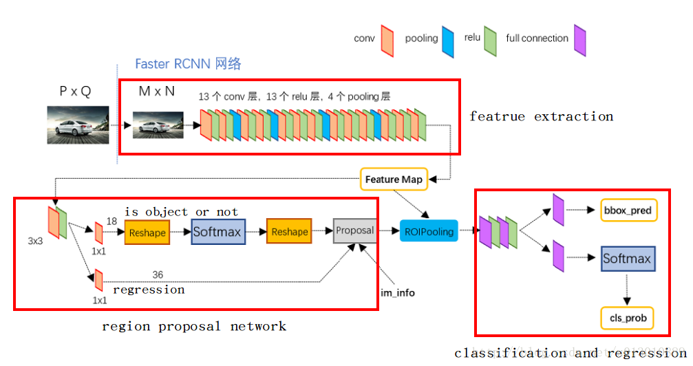
- 首先图片进行放缩到W*H,然后送入vgg16(去掉了pool5),得到feature map(W/16, H/16)
- 然后feature map上每个点都对应原图上的9个anchor,送入rpn层后输出两个: 这9个anchor前背景的概率以及4个坐标的回归
- 每个anchor经过回归后对应到原图,然后再对应到feature map经过roi pooling后输出7*7大小的map
- 最后对这个7*7的map进行分类和再次回归
(此处均为大体轮廓,具体细节见后面)
数据层
- 主要利用工厂模式适配各种数据集 factory.py中利用lambda表达式(泛函)
- 自定义适配自己数据集的类,继承于imdb
- 主要针对数据集中生成roidb,对于每个图片保持其中含有的所有的box坐标(0-index)及其类别,然后顺便保存它的面积等参数,最后记录所有图片的index及其根据index获取绝对地址的方法
# factory.py
from datasets.mydataset import mydataset
for dataset in ['xxdataset']:
  for split in ['train', 'val', 'test']:
    name = '{}_{}'.format(dataset, split)
    __sets[name] = (lambda split=split,dataset=dataset: mydataset(split, dataset))
- 1
- 2
- 3
- 4
- 5
- 6
RPN
anchors生成
经过feature extraction后,feature map的大小是(W/16, H/16), 记为(w,h),然后每个feature map每个点生成k个anchor,论文中设置了3中ratio, 3种scale 共产生了w*h*9个anchors

# # array([[ -83.,  -39.,  100.,   56.],
#       [-175.,  -87.,  192.,  104.],
#       [-359., -183.,  376.,  200.],
#       [ -55.,  -55.,   72.,   72.],
#       [-119., -119.,  136.,  136.],
#       [-247., -247.,  264.,  264.],
#       [ -35.,  -79.,   52.,   96.],
#       [ -79., -167.,   96.,  184.],
#       [-167., -343.,  184.,  360.]])
#  先以左上角(0,0)为例生成9个anchor,然后在向右向下移动,生成整个feature map所有点对应的anchor
- 1
- 2
- 3
- 4
- 5
- 6
- 7
- 8
- 9
- 10
anchors前背景和坐标预测
正如整体框架上画的那样,feature map后先跟了一个3*3的卷积,然后分别用2个1*1的卷积,预测feature map上每个点对应的9个anchor属于前背景的概率(9*2)和4个回归的坐标(9*4)
# rpn
self.rpn_net = nn.Conv2d(self._net_conv_channels, cfg.RPN_CHANNELS, [3, 3], padding=1)
self.rpn_cls_score_net = nn.Conv2d(cfg.RPN_CHANNELS, self._num_anchors * 2, [1, 1])
self.rpn_bbox_pred_net = nn.Conv2d(cfg.RPN_CHANNELS, self._num_anchors * 4, [1, 1])


rpn = F.relu(self.rpn_net(net_conv))
rpn_cls_score = self.rpn_cls_score_net(rpn) # batch * (num_anchors * 2) * h * w
rpn_bbox_pred = self.rpn_bbox_pred_net(rpn) # batch * (num_anchors * 4) * h * w
- 1
- 2
- 3
- 4
- 5
- 6
- 7
- 8
- 9
anchor target
对上一步产生的anchor分配target label,1前景or0背景or-1忽略,以便训练rpn(只有分配了label的才能计算loss,即参与训练)
无NMS
1. 对于每个gt box,找到与他iou最大的anchor然后设为正样本
2. 对于每个anchor只要它与任意一个gt box iou>0.7即设为正样本
3. 对于每个anchor它与任意一个gt box iou都<0.3即设为负样本
4. 不是正也不是负的anchor被忽略
注意
正样本的数量由num_fg = int(cfg.TRAIN.RPN_FG_FRACTION * cfg.TRAIN.RPN_BATCHSIZE)控制,默认是256*0.5=128,即最多有128个正样本参与rpn的训练. 假如正样本有1234个,则随机抽1234-128个正样本将其label设置为-1,即忽略掉,当然正样本也有可能不足128个,那就都保留下来.
负样本的数量由num_bg = cfg.TRAIN.RPN_BATCHSIZE - np.sum(labels == 1),同理如果超额也为多余的忽略.
TRAIN.RPN_FG_FRACTION控制参与rpn训练的正样本的数量
注意在RPN阶段需要的配置参数都有RPN前缀,与后面的fast rcnn的参数区别开
# Max number of foreground examples
# __C.TRAIN.RPN_FG_FRACTION = 0.5
# Total number of examples
#__C.TRAIN.RPN_BATCHSIZE = 256

# subsample positive labels if we have too many
num_fg = int(cfg.TRAIN.RPN_FG_FRACTION * cfg.TRAIN.RPN_BATCHSIZE)
fg_inds = np.where(labels == 1)[0]
if len(fg_inds) > num_fg:
  disable_inds = npr.choice(
    fg_inds, size=(len(fg_inds) - num_fg), replace=False)
  labels[disable_inds] = -1

# subsample negative labels if we have too many
num_bg = cfg.TRAIN.RPN_BATCHSIZE - np.sum(labels == 1)
bg_inds = np.where(labels == 0)[0]
if len(bg_inds) > num_bg:
  disable_inds = npr.choice(
    bg_inds, size=(len(bg_inds) - num_bg), replace=False)
  labels[disable_inds] = -1
- 1
- 2
- 3
- 4
- 5
- 6
- 7
- 8
- 9
- 10
- 11
- 12
- 13
- 14
- 15
- 16
- 17
- 18
- 19
- 20
Fast RCNN
proposal
对RPNchase的anchor进行处理,有NMS
1. 首先利用4个坐标回归值对默认的w*h*9个anchor进行坐标变换生成proposal
2. 然后利用前景概率对这些proposal进行降序排列,然后留下RPN_PRE_NMS_TOP_N个proposal 训练是留下12000,测试是留下6000
3. 对剩下的proposal进行NMS处理,阈值是0.7
4. 对于剩下的proposal,只留下RPN_POST_NMS_TOP_N,训练是2000,测试是300
最终剩下的proposal即为rois了
proposal target
对留下的proposal(train:2000, test没有这个阶段,因为测试不知道gt无法分配)分配target label,属于具体哪一个类别,以便训练后面的分类器, 下面以train阶段的某个图片为例即该张图片有2000个proposal,gt中含有15个类别的box(不含背景) (全库有20个类别)
# Minibatch size (number of regions of interest [ROIs])
# __C.TRAIN.BATCH_SIZE = 128
# Fraction of minibatch that is labeled foreground (i.e. class > 0)
# __C.TRAIN.FG_FRACTION = 0.25 控制fast rcnn中rois的正负样本比例为1:3
num_images = 1
rois_per_image = cfg.TRAIN.BATCH_SIZE / num_images # 默认为128
fg_rois_per_image = int(round(cfg.TRAIN.FG_FRACTION * rois_per_image))  # 0.25*128
- 1
- 2
- 3
- 4
- 5
- 6
- 7
- 计算每个roi(proposal)与15个gt box做iou,得到overlaps(2000, 15) ,然后选择最大的iou作为这个roi的gt label(坑点: gt box的顺序不一定和label对应,一定要取gt box的第4个维度作为label,因为可能包含15个gt box,但是全库是有20中label的)
- 然后记roi与其target label的ovlap>TRAIN.FG_THRESH(0.5)的为fg,0.1
if fg_inds.numel() > 0 and bg_inds.numel() > 0:
  fg_rois_per_image = min(fg_rois_per_image, fg_inds.numel())
  fg_inds = fg_inds[torch.from_numpy(npr.choice(np.arange(0, fg_inds.numel()), size=int(fg_rois_per_image), replace=False)).long().cuda()]
#  ......
#  主要解读npr.choice(np.arange(0, fg_inds.numel()), size=int(fg_rois_per_image), replace=False)
#  在np.arange(0, fg_inds.numel())随机取int(fg_rois_per_image)个数,replace=False不允许重复
- 1
- 2
- 3
- 4
- 5
- 6
roi pooling
上一步得到了很多大小不一的roi,对应到feature map上也是大小不一的,但是fc是需要fixed size的,于是根据SPPNet论文笔记和caffe实现说明,出来了roi pooling(spp poolingfroze 前面的卷积只更新后面的fc,why见fast rcnn的2.3段解释的)
我主要参考了这篇博客Region of interest pooling explained,但是我感觉它的示意图是有问题的,应该有overlap的
1. 我们首先根据feature map和原图的比例,把roi在原图上的坐标映射到feature map上, 然后扣出roi对应部分的feature(蓝色框为实际位置,浮点坐标(1.2,0.8)(7.2,9.7),四舍五入量化到红色框(1,1)(7,10))
int roi_start_w = round(rois_flat[index_roi + 1] * spatial_scale);  // spatial_scale 1/16
int roi_start_h = round(rois_flat[index_roi + 2] * spatial_scale);
int roi_end_w = round(rois_flat[index_roi + 3] * spatial_scale);
int roi_end_h = round(rois_flat[index_roi + 4] * spatial_scale);
- 1
- 2
- 3
- 4

2. 对红色红色框进行roipooling
float bin_size_h = (float)(roi_height) / (float)(pooled_height);  // 9/7
float bin_size_w = (float)(roi_width) / (float)(pooled_width);  // 7/7=1
for (ph = 0; ph < pooled_height; ++ph){
  for (pw = 0; pw < pooled_width; ++pw){
    int hstart = (floor((float)(ph) * bin_size_h));
    int wstart = (floor((float)(pw) * bin_size_w));
    int hend = (ceil((float)(ph + 1) * bin_size_h));
    int wend = (ceil((float)(pw + 1) * bin_size_w));
    hstart = fminf(fmaxf(hstart + roi_start_h, 0), data_height);
    hend = fminf(fmaxf(hend + roi_start_h, 0), data_height);
    wstart = fminf(fmaxf(wstart + roi_start_w, 0), data_width);
    wend = fminf(fmaxf(wend + roi_start_w, 0), data_width);
// ......
// 经过计算后w步长为1,窗口为1,没有overlap,h窗口步长不定都有overlap,注意在ph=3时窗口为3了
// 注意边界 pw=pooled_width-1时 wend=(ceil((float)(pw + 1) * bin_size_w))
//  =(ceil((float)pooled_width * (float)(roi_width) / (float)
//  =(pooled_width)))=ceil(roi_width)=roi_width
//  刚好把所有roi对应的feature map覆盖完,hend同理
//  roi_height roi_width小于pooled_height pooled_width时overlap就多一点呗
- 1
- 2
- 3
- 4
- 5
- 6
- 7
- 8
- 9
- 10
- 11
- 12
- 13
- 14
- 15
- 16
- 17
- 18
- 19

3. 对每个划分的pool bin进行max或者average pooling最后得到7*7的feature map
分类和回归
roi pooling后就得到fixed size的feature map(7*7),然后送入cls_score_net得到分类,送入bbox_pred_net粗暴的坐标回归和rpn时一样
self.cls_score_net = nn.Linear(self._fc7_channels, self._num_classes)
self.bbox_pred_net = nn.Linear(self._fc7_channels, self._num_classes * 4)
- 1
- 2
Loss采用smooth L1 Loss(和fast rcnn一致,rcnn采用的是L2 Loss)。

prior_centers = center_size(prior_boxes) #(cx, cy, w, h)
gt_centers = center_size(gt_boxes) #(cx, cy, w, h)
# tx=(gx-px)/pw  gx是gt的中心坐标x,px是proposal的中心坐标x,pw是预测的宽。ty同理
center_targets = (gt_centers[:, :2] - prior_centers[:, :2]) / prior_centers[:, 2:]
# 参照tw,th的公式
# 加了log, 降低w,h产生的loss的数量级, 让它在loss里占的比重小些, 不至于因为w,h的loss太大而让x,y产生的loss无用
# 因为若是x,y没预测准确, w,h再准确也没有用.
size_targets = torch.log(gt_centers[:, 2:]) - torch.log(prior_centers[:, 2:])
all_targets = torch.cat((center_targets, size_targets), 1)
loss = F.smooth_l1_loss(deltas, all_targets, size_average=False)/(eps + prior_centers.size(0))
- 1
- 2
- 3
- 4
- 5
- 6
- 7
- 8
- 9
- 10
smoothed L1 Loss is a robust L1 loss that is less sensitive to outliers than the L2 loss used in R-CNN and SPPnet.
上述是Fast RCNN解释为什么采用smoothed L1, 因为它对噪音点不那么敏感,即对离目标太远的点不敏感。因为L2loss求导后 0.5*(t-v)^2 求导-> (t-v) 会有一个(t-v) 的系数在,如果v离t太远梯度很容易爆炸(需要精致地调节学习率),而smoothed L1中当|t-v|>1, |t-v|-0.5 求导-> 系数是±1, 这样就避免了梯度爆炸, 也就是它更加鲁棒。(t是target,v是需要预测出来的中心xy和尺寸wh)

测试
继续假设全部类别数是20种
1. 图片送入网络后前传,没有给anchor proposal指定gt的部分(忽略_anchor_target_layer _proposal_target_layer)
2. 经过proposal得到300个roi,经过cls_score_net bbox_pred_net得到每个roi在20个类别的置信度和4个坐标回归值(可在测试时把这个回归值用上,也可以不用)
3. 测试时300个roi类别未知,所以可以对应20个类别,即有300*20个box,300*20个置信度
3. 对每一类,取300个roi>thresh(默认为0.),然后进行nms获得留下的box
4. 然后对20类留下的所有box,按概率排序,留下设定的max_per_image个box
有个不解就是为什么对于每个roi,不是选择其置信度最大的类别,而可以对应到20种类别,可能是map算法,同等置信度下,多一些box得分会高一些
for j in range(1, imdb.num_classes):
  inds = np.where(scores[:, j] > thresh)[0]
  cls_scores = scores[inds, j]
  cls_boxes = boxes[inds, j*4:(j+1)*4]
  cls_dets = np.hstack((cls_boxes, cls_scores[:, np.newaxis])) \
    .astype(np.float32, copy=False)
  keep = nms(torch.from_numpy(cls_dets), cfg.TEST.NMS).numpy() if cls_dets.size > 0 else []
  cls_dets = cls_dets[keep, :]
  all_boxes[j][i] = cls_dets
- 1
- 2
- 3
- 4
- 5
- 6
- 7
- 8
- 9
延伸
验证一下nms在训练时是不是必须的
参考An Implementation of Faster RCNN with Study for Region Sampling

• First, take the top K regions according to RPN score.
• Then, non-maximal suppression (NMS) with overlapping ratio of 0.7 is applied to perform de-duplication.
• Third, top k regions are selected as RoIs.
Intuitively, it is more likely for large regions to overlap than small regions, so large regions have a higher chance to be suppressed对这句话保留意见,nms算的是iou,没有偏向抑制大的region吧
ALL是top12000 proposal都送入后面的网络,不进行nms PRE是利用第一行已经训练好的faster rcnn直接得到最终的正负样本比例 POW: 比例和scale成反比,详细见文章。TOP是test是选择top 5000不进行nms(faster rcnn本身是选择top 6000然后nms,最后再取top300)
In fact, we find this advantage of TOP over NMS consistently exists when K is sufficiently large.