Udacity 深度学习项目２(Project2) Image Classification 解析

本项目需要搭建一个简单的卷积神经网络（CNN）来对　CIFAR-10 数据进行图片分类。本文记录了这个项目的一些注意事项。

１.数据的预处理：对于CIFAR-10　的图片数据，首先要做归一化处理。对于 Label　数据，要做 one-hot-encoder　处理。　

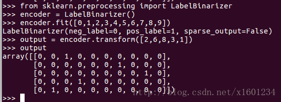
One-hot-encoder　可以利用 sklearn　中的 Preprocessing　中的 LabelBinarizer 函数：
　　　　　　这里写图片描述
　　
　　也可以利用　numpy　中的 eye　函数：
　

def one_hot_encode(x):
    """
    One hot encode a list of sample labels. Return a one-hot encoded vector for each label.
    : x: List of sample Labels
    : return: Numpy array of one-hot encoded labels
    """
    # TODO: Implement Function
    np_classes = 10
    one_hot_labels = np.eye(np_classes)[x]
    return one_hot_label

２．卷积层，最大池化层，扁平化层，全连接层，输出层的代码如下：

def conv2d_maxpool(x_tensor, conv_num_outputs, conv_ksize, conv_strides, pool_ksize, pool_strides):
    """
    Apply convolution then max pooling to x_tensor
    :param x_tensor: TensorFlow Tensor
    :param conv_num_outputs: Number of outputs for the convolutional layer
    :param conv_ksize: kernal size 2-D Tuple for the convolutional layer
    :param conv_strides: Stride 2-D Tuple for convolution
    :param pool_ksize: kernal size 2-D Tuple for pool
    :param pool_strides: Stride 2-D Tuple for pool
    : return: A tensor that represents convolution and max pooling of x_tensor
    """
    # TODO: Implement Function
    depth = x_tensor.get_shape().as_list()
    padding = 'SAME'
    conv_ksize2 = [conv_ksize[0], conv_ksize[1],depth[-1], conv_num_outputs]
    conv_strides2 = [1, conv_strides[0], conv_strides[1], 1]
    pool_ksize2 = [1, pool_ksize[0], pool_ksize[1],1]
    pool_strides2 = [1, pool_strides[0], pool_strides[1], 1]
    filter_weights = tf.Variable(tf.truncated_normal((conv_ksize2),0 ,0.1))
    filter_bias = tf.Variable(tf.zeros(conv_num_outputs))

    filter_output = tf.nn.conv2d(x_tensor, filter_weights, conv_strides2, padding)
    filter_output = tf.nn.bias_add(filter_output, filter_bias)

    filter_output = tf.nn.relu(filter_output)

    filter_output = tf.nn.max_pool(filter_output, pool_ksize2, pool_strides2, padding)
    #print (filter_output.get_shape().as_list())
    return filter_output


def flatten(x_tensor):
    """
    Flatten x_tensor to (Batch Size, Flattened Image Size)
    : x_tensor: A tensor of size (Batch Size, ...), where ... are the image dimensions.
    : return: A tensor of size (Batch Size, Flattened Image Size).
    """
    # TODO: Implement Function
    flattened_image_size = np.prod(x_tensor.get_shape().as_list()[1:])
    flat_inputs = tf.reshape(x_tensor,[-1,flattened_image_size])

    #flat_inputs = tf.contrib.layers.flatten(x_tensor)
    return flat_inputs


def fully_conn(x_tensor, num_outputs):
    """
    Apply a fully connected layer to x_tensor using weight and bias
    : x_tensor: A 2-D tensor where the first dimension is batch size.
    : num_outputs: The number of output that the new tensor should be.
    : return: A 2-D tensor where the second dimension is num_outputs.
    """
    # TODO: Implement Function
    #output = tf.contrib.layers.fully_connected(x_tensor, num_outputs)
    weights_shape = list((x_tensor.get_shape().as_list()[-1], ) + (num_outputs, ))
    weights = tf.Variable(tf.truncated_normal(weights_shape, 0, 0.1))
    bias = tf.Variable(tf.zeros(num_outputs))
    return tf.nn.relu(tf.add(tf.matmul(x_tensor, weights), bias))


def output(x_tensor, num_outputs):
    """
    Apply a output layer to x_tensor using weight and bias
    : x_tensor: A 2-D tensor where the first dimension is batch size.
    : num_outputs: The number of output that the new tensor should be.
    : return: A 2-D tensor where the second dimension is num_outputs.
    """
    # TODO: Implement Function
    image_shape = x_tensor.get_shape().as_list()[1]
    weights = tf.Variable(tf.truncated_normal([image_shape, num_outputs],0,0.01))
    bias = tf.Variable(tf.zeros(num_outputs))
    outputs = tf.add(tf.matmul(x_tensor, weights),bias)
    return outputs

３．构建模型及参数选择
　　本项目的难点在于模型的参数选择。具体参数包括：
　　　　卷积层滤波器的　size　以及 stride：
　　　　　　经过反复测试，滤波器选择　4*4，stride 选择 1 的效果较好
　　　　　　
　　　　最大池化的 size　以及 stride:
　　　　　池化的 size 选择　8*8， stride 选择１的效果较好
　　　　　
　　　　全连接层的输出 size：
　　　　　　　输出层为 384 个输出的效果较好
　　　　　　　
　　　　keep-probability:
　　　　经过测试，keep-probability 宜小一点，可以更好的防止 overfitting。但是太小的 keep-probability 也会导致运算速度慢，以及模型预测不准的问题。
　　　　
　　　　各个层级的 weight　的初始化问题：
　　　　　　　我在搭建模型初期，遇到一个很大的问题就是，初始化参数设置不合理，导致收敛太慢。一开始注意到收敛太慢的问题时，我采用的方法是增大 optimizer 的 learning-rate ，设置：
　　　　　　　

optimizer = tf.train.AdamOptimizer(learning_rate = 0.01).munimize(cost)

但是效果仍然不好。通过查询资料，发现应该在初始化变量时，调整正态分布的标准差，将默认的标准差“1”修改为 “0.1” 或 “0.01”。

最终搭建神经网络的代码如下：

def conv_net(x, keep_prob):
    """
    Create a convolutional neural network model
    : x: Placeholder tensor that holds image data.
    : keep_prob: Placeholder tensor that hold dropout keep probability.
    : return: Tensor that represents logits
    """
    # TODO: Apply 1, 2, or 3 Convolution and Max Pool layers
    #    Play around with different number of outputs, kernel size and stride
    # Function Definition from Above:
    #    conv2d_maxpool(x_tensor, conv_num_outputs, conv_ksize, conv_strides, pool_ksize, pool_strides)

    output1 = conv2d_maxpool(x, 18, (4,4),(1,1),(8,8),(1,1))
    output1 = tf.nn.dropout(output1, keep_prob)

    #output2 = conv2d_maxpool(output1,200,(2,2),(2,2),(2,2),(2,2))
    #output2 = tf.nn.dropout(output2, keep_prob)


    # TODO: Apply a Flatten Layer
    # Function Definition from Above:
    #   flatten(x_tensor)
    output3 = flatten(output1)


    # TODO: Apply 1, 2, or 3 Fully Connected Layers
    #    Play around with different number of outputs
    # Function Definition from Above:
    #   fully_conn(x_tensor, num_outputs)
    output4 = fully_conn(output3, 384)
    #output5 = fully_conn(output4,50)
    output4 = tf.nn.dropout(output4, keep_prob)

    # TODO: Apply an Output Layer
    #    Set this to the number of classes
    # Function Definition from Above:
    #   output(x_tensor, num_outputs)
    logits_output = output(output4, 10)


    # TODO: return output
    return logits_output

4.显示结果：
注意在输出结果时，计算 accuracy 要使用 validation 数据集来计算。

def print_stats(session, feature_batch, label_batch, cost, accuracy):
    """
    Print information about loss and validation accuracy
    : session: Current TensorFlow session
    : feature_batch: Batch of Numpy image data
    : label_batch: Batch of Numpy label data
    : cost: TensorFlow cost function
    : accuracy: TensorFlow accuracy function
    """
    # TODO: Implement Function

    loss = session.run(cost, feed_dict={x:feature_batch, y:label_batch, keep_prob:1.0})
    valid_acc = sess.run(accuracy, feed_dict={
                x: valid_features,
                y: valid_labels,
                keep_prob: 1.})
    print('Loss: {:>10.4f} Validation Accuracy: {:.6f}'.format(
                loss,
                valid_acc))

最终结果为，一个 batch 的准确率为 63% 左右。全部五个 batch 的准确率在 70% 左右。结果较为满意。

Udacity 深度学习项目２(Project2) Image Classification 解析

猜你喜欢