3.1 目标任务
1.学习决策树和随机森林的原理、特性
2.学习编写构造决策树的python代码
3.学习使用sklearn训练决策树和随机森林,并使用工具进行决策树可视化
3.2 实验数据
数据集:鸢尾花数据集,详情见[机器学习之回归]的Logistic回归实验
3.3 决策树特性和使用
3.3.1 决策树的特性
决策树(Decision Tree)是一种简单但广泛使用的分类器,通过训练数据建立决策树,可以高效地对未知数据进行分类。决策树有两大优点:
(1)决策树模型可读性好,具有描述性,有助于人工分析
(2)效率高,决策树只需要一次构建,反复使用,每一次预测的最大计算次数不能超过决策树的深度
决策树优点:计算复杂度不高,输出结果易于理解,对中间值的缺失不敏感,可以处理不相关的特征数据。
缺点:可能产生过度匹配问题(过拟合)
整体思路:大原则是“将无序数据变得更加有序”。从当前可供学习的数据集中,选择一个特征,根据这个特征划分出来的数据分类,可以获得最高的信息增益(在划分数据集前后信息发生的变化)。信息增益是熵的减少,或者是数据无序度的减少。在划分之后,对划分出的各个分类再次进行算法,直到所有分类中均为同一类元素,或所有特征均已使用。
3.3.2 sk-learn中决策树的使用
sklearn中提供了决策树的相关方法,即DecisionTreeClassifier分类器,它能够对数据进行多分类,具体定义及部分参数详细含义如下表所示,详细可查看项目主页(http://scikit-learn.org/stable/modules/generated/sklearn.tree.DecisionTreeClassifier.html)
| sklearn.tree.DecisionTreeClassifier class?sklearn.tree.DecisionTreeClassifier(criterion=’gini’,?splitter=’best’,?max_depth=None,?min_samples_split=2,?min_samples_leaf=1,?min_weight_fraction_leaf=0.0,?max_features=None,?random_state=None,?max_leaf_nodes=None,?min_impurity_decrease=0.0,?min_impurity_split=None,?class_weight=None,?presort=False) |
||
| 参数说明 | criterion:string | 衡量分类的质量。支持的标准有"gini"(默认)代表的是Gini impurity与"entropy"代表的是information gain |
| splitter:string | 一种在节点中选择分类的策略。支持的策略有"best"(默认)选择最好的分类和"random"选择最好的随机分类 | |
| max_depth:int or None | 树的最大深度。如果是"None"(默认),则节点会一直扩展直到所有叶子都是纯的或者所有的叶子节点都包含少于min_sample_split个样本点。忽视max_leaf_nodes是不是为Node。 | |
| persort:bool | 是否预分类数据以加速训练时最好分类的查找。在有大数据集的决策树中,如果设为true可能会减慢训练的过程。当使用一个小数据集或者一个深度受限的决策树中,可以减速训练的过程。默认False | |
和其他分类器一样,DecisionTreeClassifier有两个向量输入:X,稀疏或密集,大小为[n_sample,n_feature],存放训练样本;Y,值为整型,大小为[n_sample],存放训练样本的分类标签。但由于DecisionTreeClassifier不支持文本属性和文本标签,因此需要将原始数据集中的文本标签转化为数字标签,及X、Y应为数字矩阵。接着将X,Y传给fit()函数进行训练,得到的模型即可对样本进行预测
from sklearn import tree
X = [[0,0],[1,1]]
Y = [0,1]
#初始化
clf = tree.DecisionTreeClassifier()
#根据XY数据训练决策树
clf = clf.fit(X,Y)
#根据训练出的模型训练样本
clf.predict([[2.,2.]])
随机森林(Random Forest)
随机森林指的是利用多棵树对样本进行训练并预测的一种分类器。它通过对数据集中的子样本进行训练,从而得到多颗决策树,以提高预测的准确性并控制在单棵决策树中极易出现的过于拟合的情况。
sklearn中提供了随机森林的相关方法,即RandomForestClassifier分类器,它能够对数据进行多分类,聚体定义及部分参数详细含义如下表所示,其中很多参数都与决策树中的参数相似(页面地址:http://scikit-learn.org/stable/modules/generated/sklearn.ensemble.RandomForestClassifier.html)。
| class sklearn.ensemble.RandomForestClassifier(n_estimators=’warn’, criterion=’gini’, max_depth=None, min_samples_split=2, min_samples_leaf=1, min_weight_fraction_leaf=0.0, max_features=’auto’, max_leaf_nodes=None, min_impurity_decrease=0.0, min_impurity_split=None, bootstrap=True, oob_score=False, n_jobs=None, random_state=None, verbose=0, warm_start=False, class_weight=None) | ||
| 参数说明 | n_estimators:integer | 随机森林中的决策树的棵树,默认为0 |
| bootstrap:boolean | 在训练决策树的过程中是否使用bootstrap抽样方法,默认为True | |
| max_depth:int or None | 树的最大深度。如果是"None"(默认),则节点会一直扩展直到所有叶子都是纯的或者所有的叶子节点都包含少于min_sample_split个样本点。忽视max_leaf_nodes是不是为Node。 | |
| criterion:string | 衡量分类的质量。支持的标准有"gini"(默认)代表的是Gini impurity与"entropy"代表的是information gain | |
同样,RandomForestClassifier有两个向量输入:X,稀疏或密集,大小为[n_sample,n_feature],存放训练样本;Y,值为整型,大小为[n_sample],存放训练样本的分类标签。接着将X,Y传给fit()函数进行训练,得到的模型即可对样本进行预测
3.4 实验过程
3.4.1 实验准备
(1)确保Numpy、Matplotlib和sklearn等库已经正确安装
(2)安装graphivz工具,便于查看决策树结构(读取dot脚本写成的文本文件,做图形化显示)。Graphviz是一个开源的图形可视化软件,用于表达有向图、无向图的连接关系,它在计算机网络、生物信息、软件工程、数据库和网页设计、机器学习灯诸多领域都被技术人员广泛使用。下载地址:http://www.graphviz.org/download/
3.4.2 代码实现
(一)使用sklearn的决策树做分类
import numpy as np
import matplotlib.pyplot as plt
from sklearn import tree
def iris_type(s):
it = {'Iris-setosa':0,'Iris-versicolor':1,'Iris-virginica':2}
return it[s]
#花萼长度、花萼宽度、花瓣长度、花瓣宽度
iris_feature = 'speal length','sepal width','petal length','petsl width'
if __name__ == "__main__":
path = 'iris.data'#数据文件路径
#路径,浮点型数据,逗号分隔,第4列用函数iris_type单独处理
data = np.loadtxt(path,dtype=float,delimiter=',',converters={4:iris_type})
#将数据的0-3列组成x,第4列得到y
x,y = np.split(data,(4,),axis=1)
#为了可视化,仅使用前两列特征
x = x[:,:2]
#决策树参数估计
#min_samples_split=10#如果该节点包含的样本数目大于10,则(有可能)对其分支
#min_samples_leaf=10#若将某节点分支后,得到的每个子节点样本数目都大于10,则完成分支,否则不完成分支
clf = tree.DecisionTreeClassifier(criterion='entropy',min_samples_leaf=3)
dt_clf = clf.fit(x,y)
#保存
f = open("iris_tree.dot","w")
tree.export_graphviz(dt_clf,out_file=f)
#画图
#横纵各采样多少个值
N,M = 500,500
#得到第0列范围
x1_min,x1_max = x[:,0].min(),x[:,0].max()
#得到第1列范围
x2_min,x2_max = x[:,1].min(),x[:,1].max()
t1 = np.linspace(x1_min,x1_max,N)
t2 = np.linspace(x2_min,x2_max,M)
#生成网格采样点
x1,x2 = np.meshgrid(t1,t2)
#测试点
x_test = np.stack((x1.flat,x2.flat),axis=1)
#预测值
y_hat = dt_clf.predict(x_test)
#使之与输入形状相同
y_hat = y_hat.reshape(x1.shape)
#预测值的显示
plt.pcolormesh(x1,x2,y_hat,cmap=plt.cm.Spectral,alpha=0.1)
plt.scatter(x[:,0],x[:,1],c=np.squeeze(y),edgecolors='k',cmap=plt.cm.prism)
#显示样本
plt.xlabel(iris_feature[0])
plt.ylabel(iris_feature[1])
plt.xlim(x1_min,x1_max)
plt.ylim(x2_min,x2_max)
plt.grid()
plt.show()
#训练集上的预测结果
y_hat = dt_clf.predict(x)
y = y.reshape(-1)
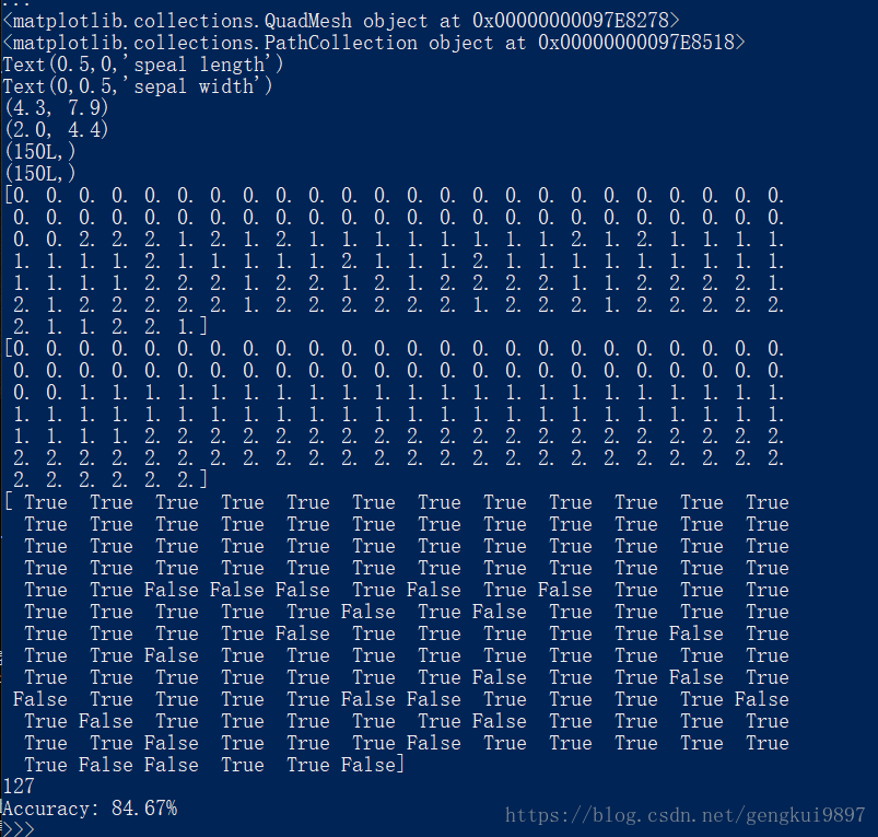
print y_hat.shape
print y.shape
result = y_hat == y
print y_hat
print y
print result
c = np.count_nonzero(result)
print c
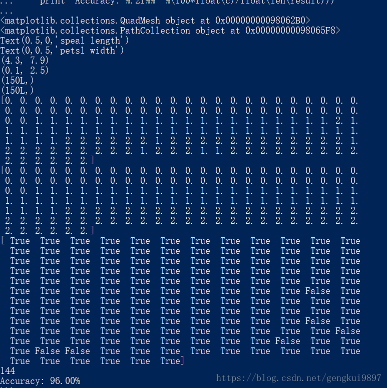
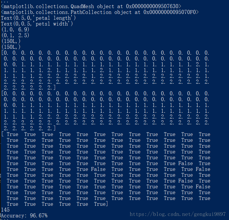
print 'Accuracy: %.2f%%' %(100*float(c)/float(len(result)))实验结果:

结果分析:
1.仅仅使用两个特征:花萼长度和花萼宽度,在150个样本中,有123个分类正确,正确率为82%。
2.使用不同特征、随机森林进行实验如下
两特征决策树:
(1)花萼长度与花瓣长度:
import numpy as np
import matplotlib.pyplot as plt
from sklearn import tree
def iris_type(s):
    it = {'Iris-setosa':0,'Iris-versicolor':1,'Iris-virginica':2}
    return it[s]

#花萼长度、花萼宽度、花瓣长度、花瓣宽度
iris_feature = 'speal length','sepal width','petal length','petsl width'
if __name__ == "__main__":
    path = 'iris.data'#数据文件路径
    #路径,浮点型数据,逗号分隔,第4列用函数iris_type单独处理
    data = np.loadtxt(path,dtype=float,delimiter=',',converters={4:iris_type})
    #将数据的0-3列组成x,第4列得到y
    x,y = np.split(data,(4,),axis=1)
    #为了可视化,仅使用前两列特征
    x = x[:,::2]
    #决策树参数估计
    #min_samples_split=10#如果该节点包含的样本数目大于10,则(有可能)对其分支
    #min_samples_leaf=10#若将某节点分支后,得到的每个子节点样本数目都大于10,则完成分支,否则不完成分支
    clf = tree.DecisionTreeClassifier(criterion='entropy',min_samples_leaf=3)
    dt_clf = clf.fit(x,y)
    #保存
    f = open("iris_tree.dot","w")
    tree.export_graphviz(dt_clf,out_file=f)
    #画图
    #横纵各采样多少个值
    N,M = 500,500
    #得到第0列范围
    x1_min,x1_max = x[:,0].min(),x[:,0].max()
    #得到第1列范围
    x2_min,x2_max = x[:,1].min(),x[:,1].max()
    t1 = np.linspace(x1_min,x1_max,N)
    t2 = np.linspace(x2_min,x2_max,M)
    #生成网格采样点
    x1,x2 = np.meshgrid(t1,t2)
    #测试点
    x_test = np.stack((x1.flat,x2.flat),axis=1)
    #预测值
    y_hat = dt_clf.predict(x_test)
    #使之与输入形状相同
    y_hat = y_hat.reshape(x1.shape)
    #预测值的显示
    plt.pcolormesh(x1,x2,y_hat,cmap=plt.cm.Spectral,alpha=0.1)
    plt.scatter(x[:,0],x[:,1],c=np.squeeze(y),edgecolors='k',cmap=plt.cm.prism)
    #显示样本
    plt.xlabel(iris_feature[0])
    plt.ylabel(iris_feature[2])
    plt.xlim(x1_min,x1_max)
    plt.ylim(x2_min,x2_max)
    plt.grid()
    plt.show()
    #训练集上的预测结果
    y_hat = dt_clf.predict(x)
    y = y.reshape(-1)
    print y_hat.shape
    print y.shape
    result = y_hat == y
    print y_hat
    print y
    print result
    c = np.count_nonzero(result)
    print c
    print 'Accuracy: %.2f%%' %(100*float(c)/float(len(result)))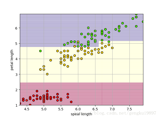

(2)花萼长度与花瓣宽度:
import numpy as np
import matplotlib.pyplot as plt
from sklearn import tree
def iris_type(s):
    it = {'Iris-setosa':0,'Iris-versicolor':1,'Iris-virginica':2}
    return it[s]

#花萼长度、花萼宽度、花瓣长度、花瓣宽度
iris_feature = 'speal length','sepal width','petal length','petsl width'
if __name__ == "__main__":
    path = 'iris.data'#数据文件路径
    #路径,浮点型数据,逗号分隔,第4列用函数iris_type单独处理
    data = np.loadtxt(path,dtype=float,delimiter=',',converters={4:iris_type})
    #将数据的0-3列组成x,第4列得到y
    x,y = np.split(data,(4,),axis=1)
    #为了可视化,仅使用前两列特征
    x = x[:,::3]
    #决策树参数估计
    #min_samples_split=10#如果该节点包含的样本数目大于10,则(有可能)对其分支
    #min_samples_leaf=10#若将某节点分支后,得到的每个子节点样本数目都大于10,则完成分支,否则不完成分支
    clf = tree.DecisionTreeClassifier(criterion='entropy',min_samples_leaf=3)
    dt_clf = clf.fit(x,y)
    #保存
    f = open("iris_tree.dot","w")
    tree.export_graphviz(dt_clf,out_file=f)
    #画图
    #横纵各采样多少个值
    N,M = 500,500
    #得到第0列范围
    x1_min,x1_max = x[:,0].min(),x[:,0].max()
    #得到第1列范围
    x2_min,x2_max = x[:,1].min(),x[:,1].max()
    t1 = np.linspace(x1_min,x1_max,N)
    t2 = np.linspace(x2_min,x2_max,M)
    #生成网格采样点
    x1,x2 = np.meshgrid(t1,t2)
    #测试点
    x_test = np.stack((x1.flat,x2.flat),axis=1)
    #预测值
    y_hat = dt_clf.predict(x_test)
    #使之与输入形状相同
    y_hat = y_hat.reshape(x1.shape)
    #预测值的显示
    plt.pcolormesh(x1,x2,y_hat,cmap=plt.cm.Spectral,alpha=0.1)
    plt.scatter(x[:,0],x[:,1],c=np.squeeze(y),edgecolors='k',cmap=plt.cm.prism)
    #显示样本
    plt.xlabel(iris_feature[0])
    plt.ylabel(iris_feature[3])
    plt.xlim(x1_min,x1_max)
    plt.ylim(x2_min,x2_max)
    plt.grid()
    plt.show()
    #训练集上的预测结果
    y_hat = dt_clf.predict(x)
    y = y.reshape(-1)
    print y_hat.shape
    print y.shape
    result = y_hat == y
    print y_hat
    print y
    print result
    c = np.count_nonzero(result)
    print c
    print 'Accuracy: %.2f%%' %(100*float(c)/float(len(result)))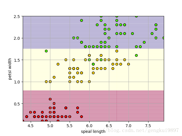
(3)花萼宽度与花瓣长度:
import numpy as np
import matplotlib.pyplot as plt
from sklearn import tree
def iris_type(s):
it = {'Iris-setosa':0,'Iris-versicolor':1,'Iris-virginica':2}
return it[s]
#花萼长度、花萼宽度、花瓣长度、花瓣宽度
iris_feature = 'speal length','sepal width','petal length','petsl width'
if __name__ == "__main__":
path = 'iris.data'#数据文件路径
#路径,浮点型数据,逗号分隔,第4列用函数iris_type单独处理
data = np.loadtxt(path,dtype=float,delimiter=',',converters={4:iris_type})
#将数据的0-3列组成x,第4列得到y
x,y = np.split(data,(4,),axis=1)
#为了可视化,仅使用前两列特征
x = x[:,1:3]
#决策树参数估计
#min_samples_split=10#如果该节点包含的样本数目大于10,则(有可能)对其分支
#min_samples_leaf=10#若将某节点分支后,得到的每个子节点样本数目都大于10,则完成分支,否则不完成分支
clf = tree.DecisionTreeClassifier(criterion='entropy',min_samples_leaf=3)
dt_clf = clf.fit(x,y)
#保存
f = open("iris_tree.dot","w")
tree.export_graphviz(dt_clf,out_file=f)
#画图
#横纵各采样多少个值
N,M = 500,500
#得到第0列范围
x1_min,x1_max = x[:,0].min(),x[:,0].max()
#得到第1列范围
x2_min,x2_max = x[:,1].min(),x[:,1].max()
t1 = np.linspace(x1_min,x1_max,N)
t2 = np.linspace(x2_min,x2_max,M)
#生成网格采样点
x1,x2 = np.meshgrid(t1,t2)
#测试点
x_test = np.stack((x1.flat,x2.flat),axis=1)
#预测值
y_hat = dt_clf.predict(x_test)
#使之与输入形状相同
y_hat = y_hat.reshape(x1.shape)
#预测值的显示
plt.pcolormesh(x1,x2,y_hat,cmap=plt.cm.Spectral,alpha=0.1)
plt.scatter(x[:,0],x[:,1],c=np.squeeze(y),edgecolors='k',cmap=plt.cm.prism)
#显示样本
plt.xlabel(iris_feature[1])
plt.ylabel(iris_feature[2])
plt.xlim(x1_min,x1_max)
plt.ylim(x2_min,x2_max)
plt.grid()
plt.show()
#训练集上的预测结果
y_hat = dt_clf.predict(x)
y = y.reshape(-1)
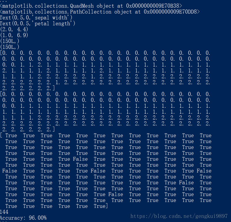
print y_hat.shape
print y.shape
result = y_hat == y
print y_hat
print y
print result
c = np.count_nonzero(result)
print c
print 'Accuracy: %.2f%%' %(100*float(c)/float(len(result)))

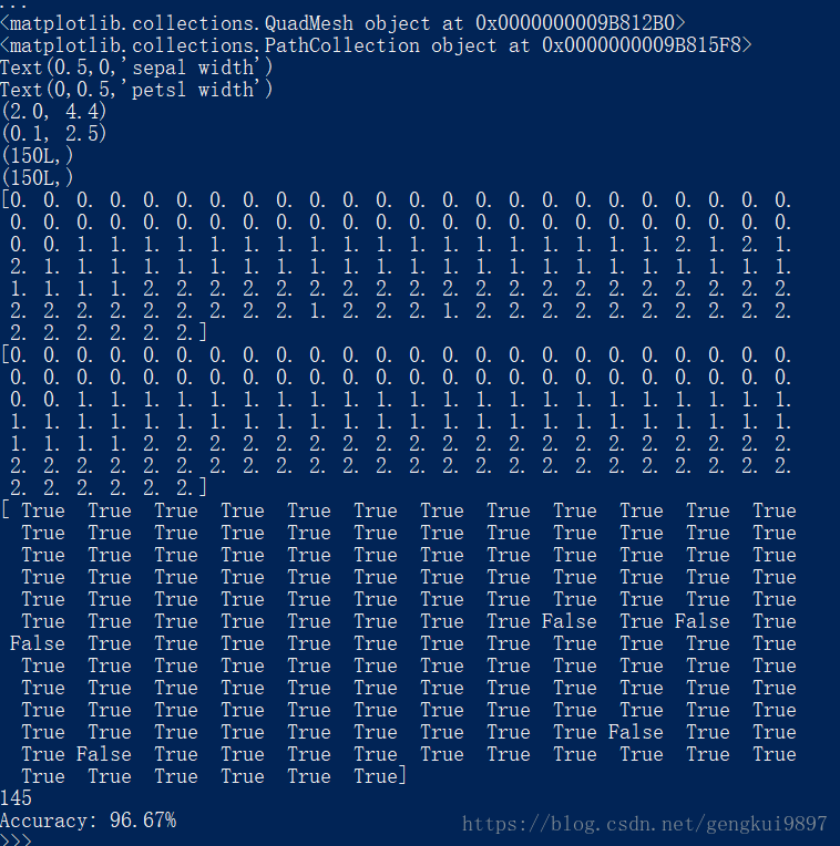
(4)花萼宽度与花瓣宽度:
import numpy as np
import matplotlib.pyplot as plt
from sklearn import tree
def iris_type(s):
    it = {'Iris-setosa':0,'Iris-versicolor':1,'Iris-virginica':2}
    return it[s]

#花萼长度、花萼宽度、花瓣长度、花瓣宽度
iris_feature = 'speal length','sepal width','petal length','petsl width'
if __name__ == "__main__":
    path = 'iris.data'#数据文件路径
    #路径,浮点型数据,逗号分隔,第4列用函数iris_type单独处理
    data = np.loadtxt(path,dtype=float,delimiter=',',converters={4:iris_type})
    #将数据的0-3列组成x,第4列得到y
    x,y = np.split(data,(4,),axis=1)
    #为了可视化,仅使用前两列特征
    x = x[:,1::2]
    #决策树参数估计
    #min_samples_split=10#如果该节点包含的样本数目大于10,则(有可能)对其分支
    #min_samples_leaf=10#若将某节点分支后,得到的每个子节点样本数目都大于10,则完成分支,否则不完成分支
    clf = tree.DecisionTreeClassifier(criterion='entropy',min_samples_leaf=3)
    dt_clf = clf.fit(x,y)
    #保存
    f = open("iris_tree.dot","w")
    tree.export_graphviz(dt_clf,out_file=f)
    #画图
    #横纵各采样多少个值
    N,M = 500,500
    #得到第0列范围
    x1_min,x1_max = x[:,0].min(),x[:,0].max()
    #得到第1列范围
    x2_min,x2_max = x[:,1].min(),x[:,1].max()
    t1 = np.linspace(x1_min,x1_max,N)
    t2 = np.linspace(x2_min,x2_max,M)
    #生成网格采样点
    x1,x2 = np.meshgrid(t1,t2)
    #测试点
    x_test = np.stack((x1.flat,x2.flat),axis=1)
    #预测值
    y_hat = dt_clf.predict(x_test)
    #使之与输入形状相同
    y_hat = y_hat.reshape(x1.shape)
    #预测值的显示
    plt.pcolormesh(x1,x2,y_hat,cmap=plt.cm.Spectral,alpha=0.1)
    plt.scatter(x[:,0],x[:,1],c=np.squeeze(y),edgecolors='k',cmap=plt.cm.prism)
    #显示样本
    plt.xlabel(iris_feature[1])
    plt.ylabel(iris_feature[3])
    plt.xlim(x1_min,x1_max)
    plt.ylim(x2_min,x2_max)
    plt.grid()
    plt.show()
    #训练集上的预测结果
    y_hat = dt_clf.predict(x)
    y = y.reshape(-1)
    print y_hat.shape
    print y.shape
    result = y_hat == y
    print y_hat
    print y
    print result
    c = np.count_nonzero(result)
    print c
    print 'Accuracy: %.2f%%' %(100*float(c)/float(len(result)))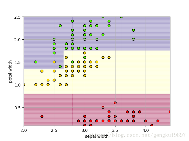
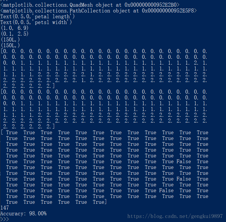
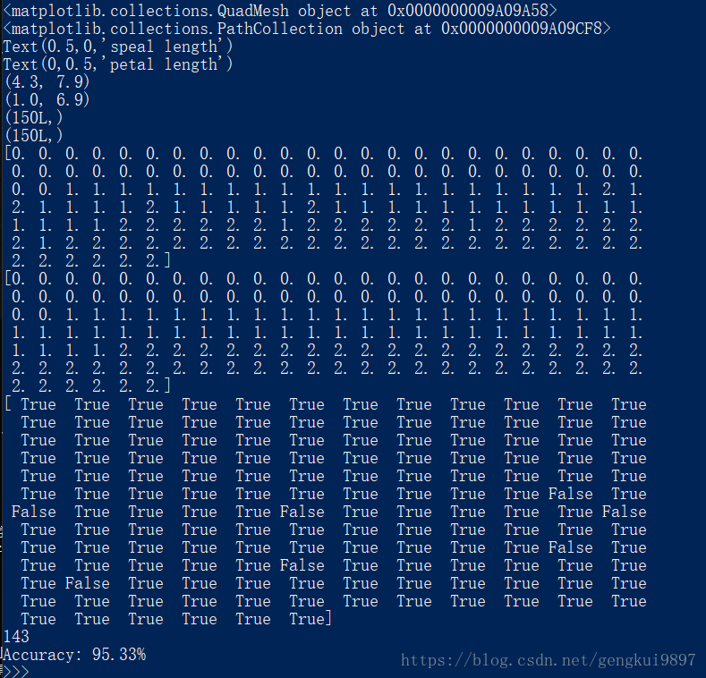
(5)花瓣长度与花瓣宽度:
import numpy as np
import matplotlib.pyplot as plt
from sklearn import tree
def iris_type(s):
    it = {'Iris-setosa':0,'Iris-versicolor':1,'Iris-virginica':2}
    return it[s]

#花萼长度、花萼宽度、花瓣长度、花瓣宽度
iris_feature = 'speal length','sepal width','petal length','petsl width'
if __name__ == "__main__":
    path = 'iris.data'#数据文件路径
    #路径,浮点型数据,逗号分隔,第4列用函数iris_type单独处理
    data = np.loadtxt(path,dtype=float,delimiter=',',converters={4:iris_type})
    #将数据的0-3列组成x,第4列得到y
    x,y = np.split(data,(4,),axis=1)
    #为了可视化,仅使用前两列特征
    x = x[:,2:4]
    #决策树参数估计
    #min_samples_split=10#如果该节点包含的样本数目大于10,则(有可能)对其分支
    #min_samples_leaf=10#若将某节点分支后,得到的每个子节点样本数目都大于10,则完成分支,否则不完成分支
    clf = tree.DecisionTreeClassifier(criterion='entropy',min_samples_leaf=3)
    dt_clf = clf.fit(x,y)
    #保存
    f = open("iris_tree.dot","w")
    tree.export_graphviz(dt_clf,out_file=f)
    #画图
    #横纵各采样多少个值
    N,M = 500,500
    #得到第0列范围
    x1_min,x1_max = x[:,0].min(),x[:,0].max()
    #得到第1列范围
    x2_min,x2_max = x[:,1].min(),x[:,1].max()
    t1 = np.linspace(x1_min,x1_max,N)
    t2 = np.linspace(x2_min,x2_max,M)
    #生成网格采样点
    x1,x2 = np.meshgrid(t1,t2)
    #测试点
    x_test = np.stack((x1.flat,x2.flat),axis=1)
    #预测值
    y_hat = dt_clf.predict(x_test)
    #使之与输入形状相同
    y_hat = y_hat.reshape(x1.shape)
    #预测值的显示
    plt.pcolormesh(x1,x2,y_hat,cmap=plt.cm.Spectral,alpha=0.1)
    plt.scatter(x[:,0],x[:,1],c=np.squeeze(y),edgecolors='k',cmap=plt.cm.prism)
    #显示样本
    plt.xlabel(iris_feature[2])
    plt.ylabel(iris_feature[3])
    plt.xlim(x1_min,x1_max)
    plt.ylim(x2_min,x2_max)
    plt.grid()
    plt.show()
    #训练集上的预测结果
    y_hat = dt_clf.predict(x)
    y = y.reshape(-1)
    print y_hat.shape
    print y.shape
    result = y_hat == y
    print y_hat
    print y
    print result
    c = np.count_nonzero(result)
    print c
    print 'Accuracy: %.2f%%' %(100*float(c)/float(len(result)))
两特征随机森林:
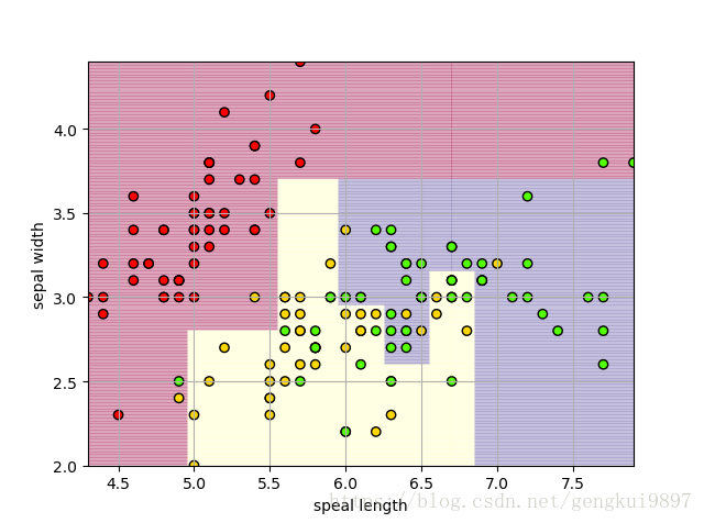
(1)花萼长度与花萼宽度:
import numpy as np
import matplotlib.pyplot as plt
from sklearn.ensemble import RandomForestClassifier
def iris_type(s):
    it = {'Iris-setosa':0,'Iris-versicolor':1,'Iris-virginica':2}
    return it[s]

#花萼长度、花萼宽度、花瓣长度、花瓣宽度
iris_feature = 'speal length','sepal width','petal length','petsl width'
if __name__ == "__main__":
    path = 'iris.data'#数据文件路径
    #路径,浮点型数据,逗号分隔,第4列用函数iris_type单独处理
    data = np.loadtxt(path,dtype=float,delimiter=',',converters={4:iris_type})
    #将数据的0-3列组成x,第4列得到y
    x,y = np.split(data,(4,),axis=1)
    #为了可视化,仅使用前两列特征
    x = x[:,:2]
    #决策树参数估计
    #min_samples_split=10#如果该节点包含的样本数目大于10,则(有可能)对其分支
    #min_samples_leaf=10#若将某节点分支后,得到的每个子节点样本数目都大于10,则完成分支,否则不完成分支
    clf = RandomForestClassifier(criterion='entropy',min_samples_leaf=3)
    dt_clf = clf.fit(x,y)
    #画图
    #横纵各采样多少个值
    N,M = 500,500
    #得到第0列范围
    x1_min,x1_max = x[:,0].min(),x[:,0].max()
    #得到第1列范围
    x2_min,x2_max = x[:,1].min(),x[:,1].max()
    t1 = np.linspace(x1_min,x1_max,N)
    t2 = np.linspace(x2_min,x2_max,M)
    #生成网格采样点
    x1,x2 = np.meshgrid(t1,t2)
    #测试点
    x_test = np.stack((x1.flat,x2.flat),axis=1)
    #预测值
    y_hat = dt_clf.predict(x_test)
    #使之与输入形状相同
    y_hat = y_hat.reshape(x1.shape)
    #预测值的显示
    plt.pcolormesh(x1,x2,y_hat,cmap=plt.cm.Spectral,alpha=0.1)
    plt.scatter(x[:,0],x[:,1],c=np.squeeze(y),edgecolors='k',cmap=plt.cm.prism)
    #显示样本
    plt.xlabel(iris_feature[0])
    plt.ylabel(iris_feature[1])
    plt.xlim(x1_min,x1_max)
    plt.ylim(x2_min,x2_max)
    plt.grid()
    plt.show()
    #训练集上的预测结果
    y_hat = dt_clf.predict(x)
    y = y.reshape(-1)
    print y_hat.shape
    print y.shape
    result = y_hat == y
    print y_hat
    print y
    print result
    c = np.count_nonzero(result)
    print c
    print 'Accuracy: %.2f%%' %(100*float(c)/float(len(result)))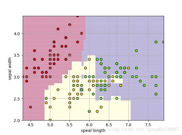
(2)花萼长度与花瓣长度:
import numpy as np
import matplotlib.pyplot as plt
from sklearn.ensemble import RandomForestClassifier
def iris_type(s):
    it = {'Iris-setosa':0,'Iris-versicolor':1,'Iris-virginica':2}
    return it[s]

#花萼长度、花萼宽度、花瓣长度、花瓣宽度
iris_feature = 'speal length','sepal width','petal length','petsl width'
if __name__ == "__main__":
    path = 'iris.data'#数据文件路径
    #路径,浮点型数据,逗号分隔,第4列用函数iris_type单独处理
    data = np.loadtxt(path,dtype=float,delimiter=',',converters={4:iris_type})
    #将数据的0-3列组成x,第4列得到y
    x,y = np.split(data,(4,),axis=1)
    #为了可视化,仅使用前两列特征
    x = x[:,::2]
    #决策树参数估计
    #min_samples_split=10#如果该节点包含的样本数目大于10,则(有可能)对其分支
    #min_samples_leaf=10#若将某节点分支后,得到的每个子节点样本数目都大于10,则完成分支,否则不完成分支
    clf = RandomForestClassifier(criterion='entropy',min_samples_leaf=3)
    dt_clf = clf.fit(x,y)
    #画图
    #横纵各采样多少个值
    N,M = 500,500
    #得到第0列范围
    x1_min,x1_max = x[:,0].min(),x[:,0].max()
    #得到第1列范围
    x2_min,x2_max = x[:,1].min(),x[:,1].max()
    t1 = np.linspace(x1_min,x1_max,N)
    t2 = np.linspace(x2_min,x2_max,M)
    #生成网格采样点
    x1,x2 = np.meshgrid(t1,t2)
    #测试点
    x_test = np.stack((x1.flat,x2.flat),axis=1)
    #预测值
    y_hat = dt_clf.predict(x_test)
    #使之与输入形状相同
    y_hat = y_hat.reshape(x1.shape)
    #预测值的显示
    plt.pcolormesh(x1,x2,y_hat,cmap=plt.cm.Spectral,alpha=0.1)
    plt.scatter(x[:,0],x[:,1],c=np.squeeze(y),edgecolors='k',cmap=plt.cm.prism)
    #显示样本
    plt.xlabel(iris_feature[0])
    plt.ylabel(iris_feature[2])
    plt.xlim(x1_min,x1_max)
    plt.ylim(x2_min,x2_max)
    plt.grid()
    plt.show()
    #训练集上的预测结果
    y_hat = dt_clf.predict(x)
    y = y.reshape(-1)
    print y_hat.shape
    print y.shape
    result = y_hat == y
    print y_hat
    print y
    print result
    c = np.count_nonzero(result)
    print c
    print 'Accuracy: %.2f%%' %(100*float(c)/float(len(result)))
(3)花萼长度与花瓣宽度:
import numpy as np
import matplotlib.pyplot as plt
from sklearn.ensemble import RandomForestClassifier
def iris_type(s):
    it = {'Iris-setosa':0,'Iris-versicolor':1,'Iris-virginica':2}
    return it[s]

#花萼长度、花萼宽度、花瓣长度、花瓣宽度
iris_feature = 'speal length','sepal width','petal length','petsl width'
if __name__ == "__main__":
    path = 'iris.data'#数据文件路径
    #路径,浮点型数据,逗号分隔,第4列用函数iris_type单独处理
    data = np.loadtxt(path,dtype=float,delimiter=',',converters={4:iris_type})
    #将数据的0-3列组成x,第4列得到y
    x,y = np.split(data,(4,),axis=1)
    #为了可视化,仅使用前两列特征
    x = x[:,::3]
    #决策树参数估计
    #min_samples_split=10#如果该节点包含的样本数目大于10,则(有可能)对其分支
    #min_samples_leaf=10#若将某节点分支后,得到的每个子节点样本数目都大于10,则完成分支,否则不完成分支
    clf = RandomForestClassifier(criterion='entropy',min_samples_leaf=3)
    dt_clf = clf.fit(x,y)
    #画图
    #横纵各采样多少个值
    N,M = 500,500
    #得到第0列范围
    x1_min,x1_max = x[:,0].min(),x[:,0].max()
    #得到第1列范围
    x2_min,x2_max = x[:,1].min(),x[:,1].max()
    t1 = np.linspace(x1_min,x1_max,N)
    t2 = np.linspace(x2_min,x2_max,M)
    #生成网格采样点
    x1,x2 = np.meshgrid(t1,t2)
    #测试点
    x_test = np.stack((x1.flat,x2.flat),axis=1)
    #预测值
    y_hat = dt_clf.predict(x_test)
    #使之与输入形状相同
    y_hat = y_hat.reshape(x1.shape)
    #预测值的显示
    plt.pcolormesh(x1,x2,y_hat,cmap=plt.cm.Spectral,alpha=0.1)
    plt.scatter(x[:,0],x[:,1],c=np.squeeze(y),edgecolors='k',cmap=plt.cm.prism)
    #显示样本
    plt.xlabel(iris_feature[0])
    plt.ylabel(iris_feature[3])
    plt.xlim(x1_min,x1_max)
    plt.ylim(x2_min,x2_max)
    plt.grid()
    plt.show()
    #训练集上的预测结果
    y_hat = dt_clf.predict(x)
    y = y.reshape(-1)
    print y_hat.shape
    print y.shape
    result = y_hat == y
    print y_hat
    print y
    print result
    c = np.count_nonzero(result)
    print c
    print 'Accuracy: %.2f%%' %(100*float(c)/float(len(result)))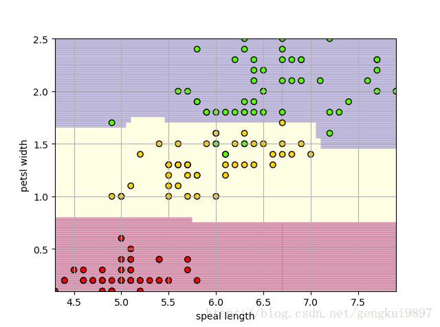

(4)花萼宽度与花瓣长度:
import numpy as np
import matplotlib.pyplot as plt
from sklearn.ensemble import RandomForestClassifier
def iris_type(s):
    it = {'Iris-setosa':0,'Iris-versicolor':1,'Iris-virginica':2}
    return it[s]

#花萼长度、花萼宽度、花瓣长度、花瓣宽度
iris_feature = 'speal length','sepal width','petal length','petsl width'
if __name__ == "__main__":
    path = 'iris.data'#数据文件路径
    #路径,浮点型数据,逗号分隔,第4列用函数iris_type单独处理
    data = np.loadtxt(path,dtype=float,delimiter=',',converters={4:iris_type})
    #将数据的0-3列组成x,第4列得到y
    x,y = np.split(data,(4,),axis=1)
    #为了可视化,仅使用前两列特征
    x = x[:,1:3]
    #决策树参数估计
    #min_samples_split=10#如果该节点包含的样本数目大于10,则(有可能)对其分支
    #min_samples_leaf=10#若将某节点分支后,得到的每个子节点样本数目都大于10,则完成分支,否则不完成分支
    clf = RandomForestClassifier(criterion='entropy',min_samples_leaf=3)
    dt_clf = clf.fit(x,y)
    #画图
    #横纵各采样多少个值
    N,M = 500,500
    #得到第0列范围
    x1_min,x1_max = x[:,0].min(),x[:,0].max()
    #得到第1列范围
    x2_min,x2_max = x[:,1].min(),x[:,1].max()
    t1 = np.linspace(x1_min,x1_max,N)
    t2 = np.linspace(x2_min,x2_max,M)
    #生成网格采样点
    x1,x2 = np.meshgrid(t1,t2)
    #测试点
    x_test = np.stack((x1.flat,x2.flat),axis=1)
    #预测值
    y_hat = dt_clf.predict(x_test)
    #使之与输入形状相同
    y_hat = y_hat.reshape(x1.shape)
    #预测值的显示
    plt.pcolormesh(x1,x2,y_hat,cmap=plt.cm.Spectral,alpha=0.1)
    plt.scatter(x[:,0],x[:,1],c=np.squeeze(y),edgecolors='k',cmap=plt.cm.prism)
    #显示样本
    plt.xlabel(iris_feature[1])
    plt.ylabel(iris_feature[2])
    plt.xlim(x1_min,x1_max)
    plt.ylim(x2_min,x2_max)
    plt.grid()
    plt.show()
    #训练集上的预测结果
    y_hat = dt_clf.predict(x)
    y = y.reshape(-1)
    print y_hat.shape
    print y.shape
    result = y_hat == y
    print y_hat
    print y
    print result
    c = np.count_nonzero(result)
    print c
    print 'Accuracy: %.2f%%' %(100*float(c)/float(len(result)))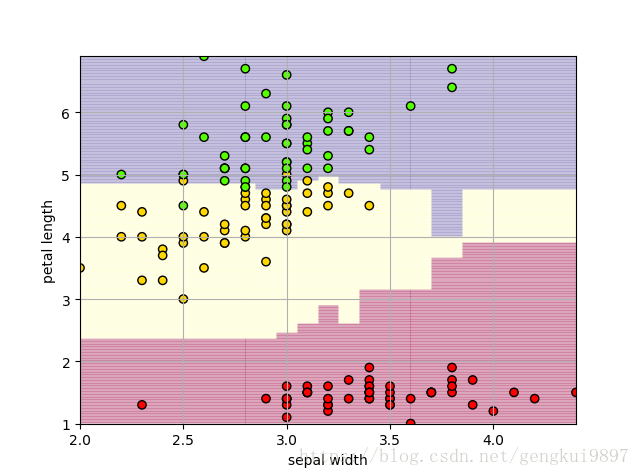
(5)花萼宽度与花瓣宽度:
import numpy as np
import matplotlib.pyplot as plt
from sklearn.ensemble import RandomForestClassifier
def iris_type(s):
it = {'Iris-setosa':0,'Iris-versicolor':1,'Iris-virginica':2}
return it[s]
#花萼长度、花萼宽度、花瓣长度、花瓣宽度
iris_feature = 'speal length','sepal width','petal length','petsl width'
if __name__ == "__main__":
path = 'iris.data'#数据文件路径
#路径,浮点型数据,逗号分隔,第4列用函数iris_type单独处理
data = np.loadtxt(path,dtype=float,delimiter=',',converters={4:iris_type})
#将数据的0-3列组成x,第4列得到y
x,y = np.split(data,(4,),axis=1)
#为了可视化,仅使用前两列特征
x = x[:,1::2]
#决策树参数估计
#min_samples_split=10#如果该节点包含的样本数目大于10,则(有可能)对其分支
#min_samples_leaf=10#若将某节点分支后,得到的每个子节点样本数目都大于10,则完成分支,否则不完成分支
clf = RandomForestClassifier(criterion='entropy',min_samples_leaf=3)
dt_clf = clf.fit(x,y)
#画图
#横纵各采样多少个值
N,M = 500,500
#得到第0列范围
x1_min,x1_max = x[:,0].min(),x[:,0].max()
#得到第1列范围
x2_min,x2_max = x[:,1].min(),x[:,1].max()
t1 = np.linspace(x1_min,x1_max,N)
t2 = np.linspace(x2_min,x2_max,M)
#生成网格采样点
x1,x2 = np.meshgrid(t1,t2)
#测试点
x_test = np.stack((x1.flat,x2.flat),axis=1)
#预测值
y_hat = dt_clf.predict(x_test)
#使之与输入形状相同
y_hat = y_hat.reshape(x1.shape)
#预测值的显示
plt.pcolormesh(x1,x2,y_hat,cmap=plt.cm.Spectral,alpha=0.1)
plt.scatter(x[:,0],x[:,1],c=np.squeeze(y),edgecolors='k',cmap=plt.cm.prism)
#显示样本
plt.xlabel(iris_feature[1])
plt.ylabel(iris_feature[3])
plt.xlim(x1_min,x1_max)
plt.ylim(x2_min,x2_max)
plt.grid()
plt.show()
#训练集上的预测结果
y_hat = dt_clf.predict(x)
y = y.reshape(-1)
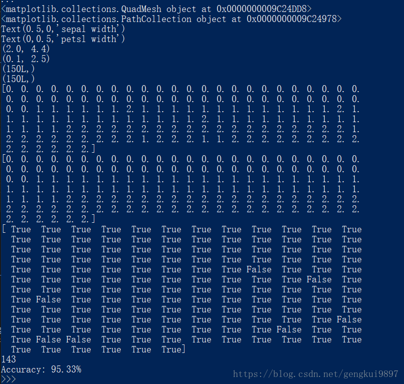
print y_hat.shape
print y.shape
result = y_hat == y
print y_hat
print y
print result
c = np.count_nonzero(result)
print c
print 'Accuracy: %.2f%%' %(100*float(c)/float(len(result)))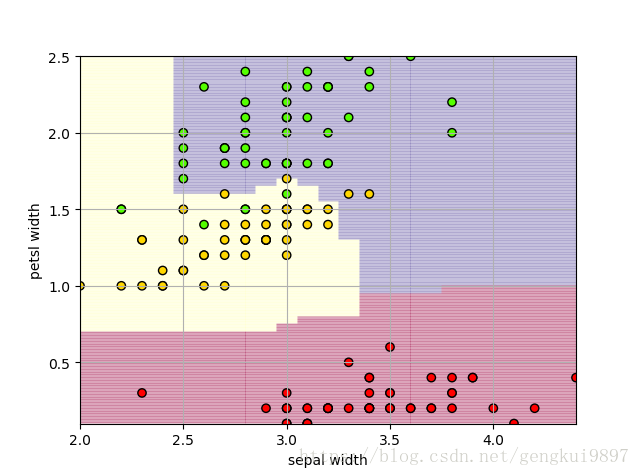
(6)花瓣长度与花瓣宽度:
import numpy as np
import matplotlib.pyplot as plt
from sklearn.ensemble import RandomForestClassifier
def iris_type(s):
    it = {'Iris-setosa':0,'Iris-versicolor':1,'Iris-virginica':2}
    return it[s]

#花萼长度、花萼宽度、花瓣长度、花瓣宽度
iris_feature = 'speal length','sepal width','petal length','petsl width'
if __name__ == "__main__":
    path = 'iris.data'#数据文件路径
    #路径,浮点型数据,逗号分隔,第4列用函数iris_type单独处理
    data = np.loadtxt(path,dtype=float,delimiter=',',converters={4:iris_type})
    #将数据的0-3列组成x,第4列得到y
    x,y = np.split(data,(4,),axis=1)
    #为了可视化,仅使用前两列特征
    x = x[:,2:4]
    #决策树参数估计
    #min_samples_split=10#如果该节点包含的样本数目大于10,则(有可能)对其分支
    #min_samples_leaf=10#若将某节点分支后,得到的每个子节点样本数目都大于10,则完成分支,否则不完成分支
    clf = RandomForestClassifier(criterion='entropy',min_samples_leaf=3)
    dt_clf = clf.fit(x,y)
    #画图
    #横纵各采样多少个值
    N,M = 500,500
    #得到第0列范围
    x1_min,x1_max = x[:,0].min(),x[:,0].max()
    #得到第1列范围
    x2_min,x2_max = x[:,1].min(),x[:,1].max()
    t1 = np.linspace(x1_min,x1_max,N)
    t2 = np.linspace(x2_min,x2_max,M)
    #生成网格采样点
    x1,x2 = np.meshgrid(t1,t2)
    #测试点
    x_test = np.stack((x1.flat,x2.flat),axis=1)
    #预测值
    y_hat = dt_clf.predict(x_test)
    #使之与输入形状相同
    y_hat = y_hat.reshape(x1.shape)
    #预测值的显示
    plt.pcolormesh(x1,x2,y_hat,cmap=plt.cm.Spectral,alpha=0.1)
    plt.scatter(x[:,0],x[:,1],c=np.squeeze(y),edgecolors='k',cmap=plt.cm.prism)
    #显示样本
    plt.xlabel(iris_feature[2])
    plt.ylabel(iris_feature[3])
    plt.xlim(x1_min,x1_max)
    plt.ylim(x2_min,x2_max)
    plt.grid()
    plt.show()
    #训练集上的预测结果
    y_hat = dt_clf.predict(x)
    y = y.reshape(-1)
    print y_hat.shape
    print y.shape
    result = y_hat == y
    print y_hat
    print y
    print result
    c = np.count_nonzero(result)
    print c
    print 'Accuracy: %.2f%%' %(100*float(c)/float(len(result)))
(二)使用sklearn的决策树做回归
import numpy as np
from sklearn.tree import DecisionTreeRegressor as dtr
import  matplotlib.pyplot as plt

N = 100
#[-3,3)
x = np.random.rand(N)*6-3
x.sort()
y = np.sin(x) + np.random.randn(N)*0.05
#转置后,得到N个样本,每个样本都是一维的
x = x.reshape(-1,1)
#比较决策树的深度
depth = [2,4,6,8,10]
clr = 'rgmby'
reg = [dtr(criterion='mse',max_depth=depth[0]),
 dtr(criterion='mse',max_depth=depth[1]),
 dtr(criterion='mse',max_depth=depth[2]),
 dtr(criterion='mse',max_depth=depth[3]),
 dtr(criterion='mse',max_depth=depth[4])]
plt.plot(x,y,'ko',linewidth=2,label='Actual')
x_test = np.linspace(-3,3,50).reshape(-1,1)
for i,r in enumerate(reg):
    dt = r.fit(x,y)
    y_hat = dt.predict(x_test)
    plt.plot(x_test,y_hat,'-',color=clr[i],linewidth=2,label='Depth=%d' %depth[i])

plt.legend(loc='upper left')
plt.grid()
plt.show()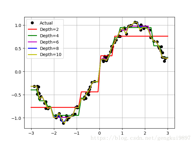
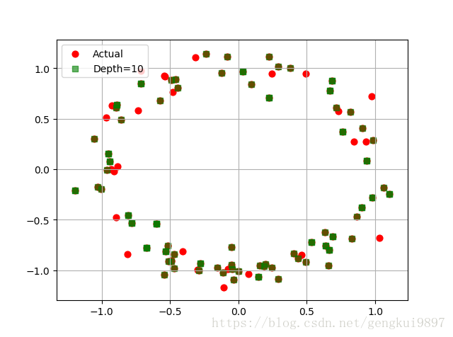
(三)决策树多输出预测
import numpy as np
from sklearn.tree import DecisionTreeRegressor as dtr
import  matplotlib.pyplot as plt

N = 100
#[-4,4)
x = np.random.rand(N)*8-4
x.sort()
y1 = np.sin(x) + np.random.randn(N)*0.1
y2 = np.cos(x) + np.random.randn(N)*0.1
y = np.vstack((y1,y2)).T
#转置后,得到N个样本,每个样本都是一维的
x = x.reshape(-1,1)
depth = 10
reg = dtr(criterion='mse',max_depth=depth)
dt = reg.fit(x,y)
x_test = np.linspace(-4,4,num=100).reshape(-1,1)
y_hat = dt.predict(x_test)
plt.scatter(y[:,0],y[:,1],c='r',s=40,label='Actual')
plt.scatter(y_hat[:,0],y_hat[:,1],c='g',marker='s',s=40,label='Depth=%d' %depth,alpha=0.6)
plt.legend(loc='upper left')
plt.grid()
plt.show()