版权声明:https://blog.csdn.net/thfyshz版权所有 https://blog.csdn.net/thfyshz/article/details/83650174
时间序列
resample函数的用法:
In [14]: rng = pd.date_range('1/1/2012', periods=100, freq='S')
In [15]: ts = pd.Series(np.random.randint(0, 500, len(rng)), index=rng)
#以五分钟为间隔,并加总。由于是随机生成的,所以每次结果可能不同
In [16]: ts.resample('5Min').sum()
Out[16]:
2012-01-01    25820
Freq: 5T, dtype: int32

In [17]: ttt = pd.date_range('1/1/2017', periods=12, freq='T')
In [18]: sss = pd.Series(range(12), index=ttt)
In [19]: sss
Out[19]:
2017-01-01 00:00:00     0
2017-01-01 00:01:00     1
2017-01-01 00:02:00     2
2017-01-01 00:03:00     3
2017-01-01 00:04:00     4
2017-01-01 00:05:00     5
2017-01-01 00:06:00     6
2017-01-01 00:07:00     7
2017-01-01 00:08:00     8
2017-01-01 00:09:00     9
2017-01-01 00:10:00    10
2017-01-01 00:11:00    11
Freq: T, dtype: int64
# 此间隔与下一个间隔之间的值的和
In [21]: sss.resample('3T').sum()
Out[21]:
2017-01-01 00:00:00     3
2017-01-01 00:03:00    12
2017-01-01 00:06:00    21
2017-01-01 00:09:00    30
Freq: 3T, dtype: int64
利用tz_localize和tz_convert函数转化时区:
In [111]: rng = pd.date_range('3/6/2012 00:00', periods=5, freq='D')
In [112]: ts = pd.Series(np.random.randn(len(rng)), rng)
In [113]: ts
Out[113]:
2012-03-06    0.464000
2012-03-07    0.227371
2012-03-08   -0.496922
2012-03-09    0.306389
2012-03-10   -2.290613
Freq: D, dtype: float64

# 定位时区
In [114]: ts_utc = ts.tz_localize('UTC')
In [115]: ts_utc
Out[115]:
2012-03-06 00:00:00+00:00    0.464000
2012-03-07 00:00:00+00:00    0.227371
2012-03-08 00:00:00+00:00   -0.496922
2012-03-09 00:00:00+00:00    0.306389
2012-03-10 00:00:00+00:00   -2.290613
Freq: D, dtype: float64

#转换时区,参数也可为'America/New_York'
In [116]: ts_utc.tz_convert('US/Eastern')
Out[116]:
2012-03-05 19:00:00-05:00    0.464000
2012-03-06 19:00:00-05:00    0.227371
2012-03-07 19:00:00-05:00   -0.496922
2012-03-08 19:00:00-05:00    0.306389
2012-03-09 19:00:00-05:00   -2.290613
Freq: D, dtype: float64
不同时间类型的转化,参考Python时间转换:
In [117]: rng = pd.date_range('1/1/2012', periods=5, freq='M')
In [118]: ts = pd.Series(np.random.randn(len(rng)), index=rng)
In [119]: ts
Out[119]:
2012-01-31   -1.134623
2012-02-29   -1.561819
2012-03-31   -0.260838
2012-04-30    0.281957
2012-05-31    1.523962
Freq: M, dtype: float64

In [120]: ps = ts.to_period()
In [121]: ps
Out[121]:
2012-01   -1.134623
2012-02   -1.561819
2012-03   -0.260838
2012-04    0.281957
2012-05    1.523962
Freq: M, dtype: float64

In [122]: ps.to_timestamp()
Out[122]:
2012-01-01   -1.134623
2012-02-01   -1.561819
2012-03-01   -0.260838
2012-04-01    0.281957
2012-05-01    1.523962
Freq: MS, dtype: float64
In [123]: prng = pd.period_range('1990Q1', '2000Q4', freq='Q-NOV')

In [124]: ts = pd.Series(np.random.randn(len(prng)), prng)

In [125]: ts.index = (prng.asfreq('M', 'e') + 1).asfreq('H', 's') + 9

In [126]: ts.head()
Out[126]:
1990-03-01 09:00   -0.902937
1990-06-01 09:00    0.068159
1990-09-01 09:00   -0.057873
1990-12-01 09:00   -0.368204
1991-03-01 09:00   -1.144073
Freq: H, dtype: float64
分类
In [127]: df = pd.DataFrame({"id":[1,2,3,4,5,6], "raw_grade":['a', 'b', 'b', 'a', 'a', 'e']})
In [128]: df["grade"] = df["raw_grade"].astype("category")

In [129]: df["grade"]
Out[129]:
0    a
1    b
2    b
3    a
4    a
5    e
Name: grade, dtype: category
Categories (3, object): [a, b, e]

In [130]: df["grade"].cat.categories = ["very good", "good", "very bad"]

In [131]: df["grade"] = df["grade"].cat.set_categories(["very bad", "bad", "medium", "good", "very good"])

In [132]: df["grade"]
Out[132]:
0    very good
1         good
2         good
3    very good
4    very good
5     very bad
Name: grade, dtype: category
Categories (5, object): [very bad, bad, medium, good, very good]

In [133]: df.sort_values(by="grade")
Out[133]:
   id raw_grade      grade
5   6         e   very bad
1   2         b       good
2   3         b       good
0   1         a  very good
3   4         a  very good
4   5         a  very good

In [134]: df.groupby("grade").size()
Out[134]:
grade
very bad     1
bad          0
medium       0
good         2
very good    3
dtype: int64
画图
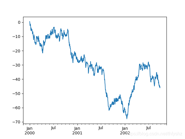
随机游走并累计加总:
In [135]: ts = pd.Series(np.random.randn(1000), index=pd.date_range('1/1/2000', periods=1000))
In [136]: ts = ts.cumsum()
In [137]: ts.plot()
Out[137]: <matplotlib.axes._subplots.AxesSubplot at 0x7f213444c048>
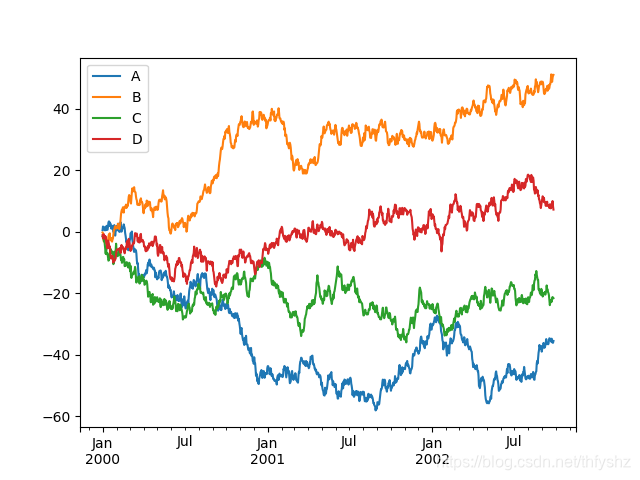
In [138]: df = pd.DataFrame(np.random.randn(1000, 4), index=ts.index,
   .....:                   columns=['A', 'B', 'C', 'D'])
   .....:
In [139]: df = df.cumsum()
In [140]: plt.figure(); df.plot(); plt.legend(loc='best')
Out[140]: <matplotlib.legend.Legend at 0x7f212489a780>
导入与导出
简单了解即可:
In [145]: df.to_excel('foo.xlsx', sheet_name='Sheet1')
In [146]: pd.read_excel('foo.xlsx', 'Sheet1', index_col=None, na_values=['NA'])