论文解读|【Densenet】密集连接的卷积网络（附Pytorch代码讲解）

版权声明：本文为王小草原创文章，要转载请先联系本人哦 https://blog.csdn.net/sinat_33761963/article/details/83958802

---

@[t oc]

1 简单介绍

论文题目：Densely Connected Convolutional Networks
发表机构：康奈尔大学，清华大学，Facebook AI
发表时间：2018年1月
论文代码：https://github.com/WangXiaoCao/attention-is-all-you-need-pytorch
pytorch代码：https://github.com/WangXiaoCao/attention-is-all-you-need-pytorch

1.1 背景介绍

1.卷积神经网络CNN在计算机视觉物体识别上优势显著，典型的模型有：LeNet5, VGG, Highway Network, Residual Network.

2.CNN越深则效果越好，但是，会面临梯度弥散的问题，经过层数越多，则前面的信息就会渐渐减弱和消散。

3.目前已有很多措施去解决以上困境：
（1）Highway Network,Residual Network通过前后两层的残差链接使信息尽量不丢失
（2）Stochastic depth通过随机drop掉Resnet的一些层来缩短模型
（3）FractalNets通过重复组合一些平行的层序列来保证深度的同时减轻这个问题。
但这些措施都有一个共性：都是在前一层和后一层中都建立一个短连接。比如，酱紫：

1.2 本文概要

1.2.1 模型结构预览

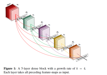
本文提出的densenet就更霸道了，为了确保网络中最大的信息流通，让每层都与改层之前的所有层都相连，即每层的输入，是前面所有层的输出的concat.(resnet用的是sum).整体结构是酱紫的：

1.2.2 优点

1.需要更少参数。

2.使得信息（前向计算时）或梯度（后向计算时）在整个网络中的保持地更好，可以训练更深的模型。

3.dense connection有正则化的效果，在较少训练集上减少过拟合。

扫描二维码关注公众号，回复： 4258349 查看本文章

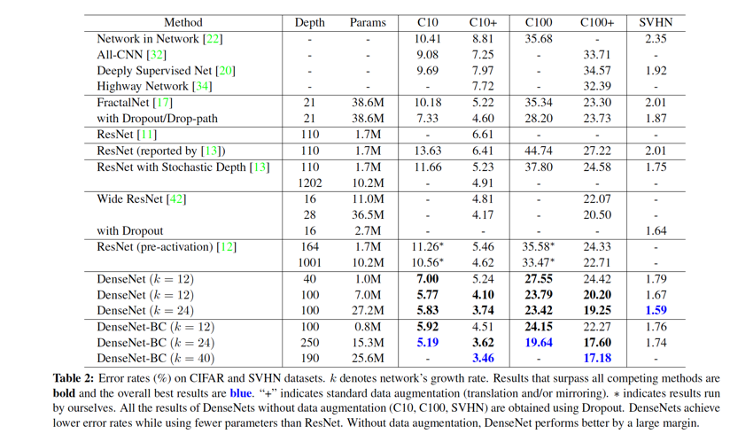
1.2.3 实验结果

在4个benchmark datasets (CIFAR-10, CIFAR-100, SVHN, and
ImageNet)上测试。
大部分任务上都优于state of art.

2 模型结构

2.1 整体结构

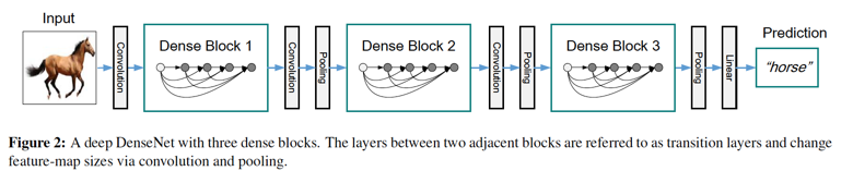
1.输入：图片
2.经过feature block（图中的第一个convolution层，后面可以加一个pooling层,这里没有画出来）
3.经过第一个dense block， 该Block中有n个dense layer,灰色圆圈表示，每个dense layer都是dense connection,即每一层的输入都是前面所有层的输出的拼接
4.经过第一个transition block,由convolution和poolling组成
5.经过第二个dense block
6.经过第二个transition block
7.经过第三个dense block
8.经过classification block,由pooling,linear层组成，输出softmax的score
9.经过prediction层，softmax分类
10.输出：分类概率

作者在4个数据集上进行测试，CIFAR-10, CIFAR-100, SVHN上构建的是以上3个dense block + 2个transition block；在ImageNet上构建的是4个dense block + 3个transition block。两者在参数的设置上略有不同，下文将以ImageNet上构建的densenet为例进行讲解。

2.2 Feature Block

Feature Block是输入层与第一个Dense Block之间的那一部分，上面结构图中只画了一个卷积，在ImageNet数据集上构建的densenet中其实后面还跟了一个poolling层。计算过程如下：

输入：图片 （244 * 244 * 3）
1.卷积层convolution计算：in_channel=3, out_channel=64,kernel_size=7,stride=2,padding=3，输出（122 * 122 * 64）
2.batch normalization计算，输入与输出维度不变 （122 * 122 * 64）
3.激活函数relu计算，输入与输出维度不变 （122 * 122 * 64）
4.池化层poollig计算，kenel_size=3, stride=2,padding=1，输出（56 * 56 * 64）

    from torch.nn import Sequential, Conv2d, BatchNorm2d, ReLU, MaxPool2d
    
    class FeatureBlock(RichRepr, Sequential):
        def __init__(self, in_channels, out_channels):
            super(FeatureBlock, self).__init__()
    
            self.in_channels = in_channels
            self.out_channels = out_channels
    
            # add_module:在现有model中增添子module
            self.add_module('conv', Conv2d(in_channels, out_channels, kernel_size=7, stride=2, padding=3, bias=False)),
            self.add_module('norm', BatchNorm2d(out_channels)),
            self.add_module('relu', ReLU(inplace=True)),
            self.add_module('pool', MaxPool2d(kernel_size=3, stride=2, padding=1)),

2.3 Dense Block 和 Dense Layer

2.3.1 Dense Layer

一个Dense Block中是由L层dense laryer组成，layer之间是dense connectivity。从下面这个公式上来体会什么是dense connectivity，第l层的输出是：

H_l是该layer的计算函数，输入是x0到x_l-1的拼接，即模型的原始输出(x0)和前面每层的输出的拼接。这个拼接是channel维度上的拼接，即维度（56 * 56 * 64）的数据 和（56 * 56 * 32）的数据拼接成（56 * 56 * 96）的数据维度。

而ResNet就不同了,是直接将前一层的输出加在该层的输出之上：

Dense Layer中函数H(·)的计算过程如下（括号中的数据维度是以第一个dense block的第一个dense layer为例的，整个模型的k值是预先设定的，本模型为k=32）：

输入：Feature Block的输出（56 * 56 * 64）或者是上一层dense layer的输出
1.Batch Normalization， 输出（56 * 56 * 64）
2.ReLU ，输出（56 * 56 * 64）
3.Bottleneck，是可选的，为了减少 feature-maps的数量，过程如下3步
-1x1 Convolution, kernel_size=1, channel = 4k, 则输出为（56 * 56 * 128）
-Batch Normalization（56 * 56 * 128）
-ReLU（56 * 56 * 128）
4.Convolution, kernel_size=3, channel = k （56 * 56 * 32）
5.Dropout,可选的,用于防止过拟合（56 * 56 * 32）

from typing import Optional
from torch.nn import Sequential, BatchNorm2d, ReLU, Conv2d, Dropout2d
from .bottleneck import Bottleneck

class DenseLayer(RichRepr, Sequential):
    r"""
    Dense Layer as described in [DenseNet](https://arxiv.org/abs/1608.06993)
    and implemented in https://github.com/liuzhuang13/DenseNet

    Consists of:

    - Batch Normalization
    - ReLU
    - (Bottleneck)
    - 3x3 Convolution
    - (Dropout)
    """

    def __init__(self, in_channels: int, out_channels: int,
                 bottleneck_ratio: Optional[int] = None, dropout: float = 0.0):
        super(DenseLayer, self).__init__()

        self.in_channels = in_channels
        self.out_channels = out_channels

        self.add_module('norm', BatchNorm2d(num_features=in_channels))
        self.add_module('relu', ReLU(inplace=True))

        if bottleneck_ratio is not None:
            self.add_module('bottleneck', Bottleneck(in_channels, bottleneck_ratio * out_channels))
            in_channels = bottleneck_ratio * out_channels

        self.add_module('conv', Conv2d(in_channels, out_channels, kernel_size=3, padding=1, bias=False))

        if dropout > 0:
            self.add_module('drop', Dropout2d(dropout, inplace=True))

Bottleneck代码如下：

from torch.nn import Sequential, Conv2d, BatchNorm2d, ReLU

from ..utils import RichRepr


class Bottleneck(RichRepr, Sequential):
    r"""
    A 1x1 convolutional layer, followed by Batch Normalization and ReLU
    """

    def __init__(self, in_channels: int, out_channels: int):
        super(Bottleneck, self).__init__()

        self.in_channels = in_channels
        self.out_channels = out_channels

        self.add_module('conv', Conv2d(in_channels, out_channels, kernel_size=1, bias=False))
        self.add_module('norm', BatchNorm2d(num_features=out_channels))
        self.add_module('relu', ReLU(inplace=True))

2.3.2 Dense Block

Dense Block有L层dense layer组成
layer 0:输入（56 * 56 * 64）->输出（56 * 56 * 32）
layer 1:输入（56 * 56 (32 * 1))->输出（56 * 56 * 32）
layer 2:输入（56 * 56 (32 * 2))->输出（56 * 56 * 32）
…
layer L:输入（56 * 56 * (32 * L))->输出（56 * 56 * 32）

注意，L层dense layer的输出都是不变的，而每层的输入channel数是增加的，因为如上所述，每层的输入是前面所有层的拼接。

rom typing import Optional
import torch
from torch.nn import Module
from .dense_layer import DenseLayer

class DenseBlock(RichRepr, Module):
    r"""
    Dense Block as described in [DenseNet](https://arxiv.org/abs/1608.06993)
    and implemented in https://github.com/liuzhuang13/DenseNet

    - Consists of several DenseLayer (possibly using a Bottleneck and Dropout) with the same output shape
    - The first DenseLayer is fed with the block input
    - Each subsequent DenseLayer is fed with a tensor obtained by concatenating the input and the output
      of the previous DenseLayer on the channel axis
    - The block output is the concatenation of the output of every DenseLayer, and optionally the block input,
      so it will have a channel depth of (growth_rate * num_layers) or (growth_rate * num_layers + in_channels)
    """

    def __init__(self, in_channels: int, growth_rate: int, num_layers: int,
                 concat_input: bool = False, dense_layer_params: Optional[dict] = None):
        super(DenseBlock, self).__init__()

        self.concat_input = concat_input
        self.in_channels = in_channels
        self.growth_rate = growth_rate
        self.num_layers = num_layers
        self.out_channels = growth_rate * num_layers
        if self.concat_input:
            self.out_channels += self.in_channels

        if dense_layer_params is None:
            dense_layer_params = {}

        for i in range(num_layers):
            # 增添dense_layer:norm->relu->bottleneck->conv->dropout
            self.add_module(
                f'layer_{i}',
                DenseLayer(in_channels=in_channels + i * growth_rate, out_channels=growth_rate, **dense_layer_params)
            )

    def forward(self, block_input):
        layer_input = block_input
        # empty tensor (not initialized) + shape=(0,)
        layer_output = block_input.new_empty(0)

        all_outputs = [block_input] if self.concat_input else []
        for layer in self._modules.values():
            layer_input = torch.cat([layer_input, layer_output], dim=1)
            layer_output = layer(layer_input)
            all_outputs.append(layer_output)

        return torch.cat(all_outputs, dim=1)

2.4 Transition Block

Transition Block是在两个Dense Block之间的，由一个卷积+一个pooling组成（下面的数据维度以第一个transition block为例）：

输入：Dense Block的输出（56 * 56 * 32）
1.Batch Normalization 输出（56 * 56 * 32）
2.ReLU 输出（56 * 56 * 32）
3.1x1 Convolution，kernel_size=1，此处可以根据预先设定的压缩系数（0-1之间）来压缩原来的channel数,以减小参数，输出（56 * 56 *(32 * compression)）
4.2x2 Average Pooling 输出（28 * 28 * (32 * compression)）

class Transition(RichRepr, Sequential):
    r"""
    Transition Block as described in [DenseNet](https://arxiv.org/abs/1608.06993)
    and implemented in https://github.com/liuzhuang13/DenseNet

    Consists of:
    - Batch Normalization
    - ReLU
    - 1x1 Convolution (with optional compression of the number of channels)
    - 2x2 Average Pooling
    """

    def __init__(self, in_channels, compression: float = 1.0):
        super(Transition, self).__init__()
        if not 0.0 < compression <= 1.0:
            raise ValueError(f'Compression must be in (0, 1] range, got {compression}')

        self.in_channels = in_channels
        # transition中可设置压缩系数，以减少输出channel
        self.out_channels = int(ceil(compression * in_channels))

        self.add_module('norm', BatchNorm2d(num_features=self.in_channels))
        self.add_module('relu', ReLU(inplace=True))
        self.add_module('conv', Conv2d(self.in_channels, self.out_channels, kernel_size=1, bias=False))
        self.add_module('pool', AvgPool2d(kernel_size=2, stride=2))

2.5 循环Dense Block和Transition

论文中，在ImageNet的数据集上，构建的densenet是由4个Dense Block，和3个Transition构成，按照上文讲述的过程，数据流的演变过程应该是：

Dense Block1：输入（565664）,输出（565632）
Transition1：输入（565632）,输出（282832）
Dense Block2：输入（282832）,输出（282832）
Transition2：输入（282832）,输出（141432）
Dense Block3：输入（141432）,输出（141432）
Transition3：输入（141432）,输出（7732）

2.6 ClassificationBlock

最后一步是ClassificationBlock，这一步将原来3维的数据拉平成一维，再接上全连接层，以准备做softmax。计算过程如下：

输入：Transition3的输出（7 * 7 * 32）
1.Batch Normalization, 输出（7 * 7 * 32）
2.ReLU, 输出（7 * 7 * 32）
3.poolling, kernel_size=7, stride=1,输出（1 * 1 * 32）
4.flatten,将（1 * 1 * 32）铺平成（1 * 32）
5.Linear全连接，输出（1*classes_num) classes_num为待分类的数目

from torch.nn import Sequential, BatchNorm2d, ReLU, AvgPool2d, Linear
from ..shared import Flatten

class ClassificationBlock(RichRepr, Sequential):
    r"""
    Classification block for [DenseNet](https://arxiv.org/abs/1608.06993),
    takes in a 7x7 feature map and outputs logit scores for classification
    """

    def __init__(self, in_channels, output_classes):
        super(ClassificationBlock, self).__init__()

        self.in_channels = in_channels
        self.out_classes = output_classes

        self.add_module('norm', BatchNorm2d(num_features=in_channels))
        self.add_module('relu', ReLU(inplace=True))
        self.add_module('pool', AvgPool2d(kernel_size=7, stride=1))
        self.add_module('flatten', Flatten())
        self.add_module('linear', Linear(in_channels, output_classes))

flaten代码如下：

from torch.nn import Module

class Flatten(Module):
    def forward(self, x):
        return x.view(x.size(0), -1)

最后将以上输出进入softmax，预测每个类别的概率。

logits = self(x)  //x是linear层的输出
return F.softmax(logits)

2.7 整合以上过程

将以上所有过程都这个起来，构建一个完整的densenet模型，代码如下：

from itertools import zip_longest
from typing import Sequence, Union, Optional
from torch.nn import Sequential, Conv2d, BatchNorm2d, Linear, init
from torch.nn import functional as F
from .classification_block import ClassificationBlock
from .feature_block import FeatureBlock
from .transition import Transition
from ..shared import DenseBlock


# 继承Sequential类
class DenseNet(Sequential):
    def __init__(self,
                 in_channels: int = 3,
                 output_classes: int = 1000,
                 initial_num_features: int = 64,
                 dropout: float = 0.0,

                 dense_blocks_growth_rates: Union[int, Sequence[int]] = 32,
                 dense_blocks_bottleneck_ratios: Union[Optional[int], Sequence[Optional[int]]] = 4,
                 dense_blocks_num_layers: Union[int, Sequence[int]] = (6, 12, 24, 16),
                 transition_blocks_compression_factors: Union[float, Sequence[float]] = 0.5):
        """
        构建完成densenet模型
        :param in_channels: 输入的channel数目
        :param output_classes: 待分类别树
        :param initial_num_features: 进入第一个Block的feature map数目
        :param dropout: dropout的比率
        :param dense_blocks_growth_rates: k（block中的channel数）
        :param dense_blocks_bottleneck_ratios: （bottleneck的比率）
        :param dense_blocks_num_layers: densenet的block数目
        :param transition_blocks_compression_factors: 在transition层中的压缩系数（0-1之间）
        """
        super(DenseNet, self).__init__()

        # region Parameters handling
        self.in_channels = in_channels
        self.output_classes = output_classes

        # 扩展成4维：（10，10，10，10）
        if type(dense_blocks_growth_rates) == int:
            dense_blocks_growth_rates = (dense_blocks_growth_rates,) * 4
        if dense_blocks_bottleneck_ratios is None or type(dense_blocks_bottleneck_ratios) == int:
            dense_blocks_bottleneck_ratios = (dense_blocks_bottleneck_ratios,) * 4
        if type(dense_blocks_num_layers) == int:
            dense_blocks_num_layers = (dense_blocks_num_layers,) * 4
        if type(transition_blocks_compression_factors) == float:
            transition_blocks_compression_factors = (transition_blocks_compression_factors,) * 3
        # endregion

        # region First convolution
        # 1.第一个卷积：covn->norm->relu->pool
        features = FeatureBlock(in_channels, initial_num_features)
        current_channels = features.out_channels
        self.add_module('features', features)
        # endregion

        # region Dense Blocks and Transition layers
        # Dense Blocks 参数
        dense_blocks_params = [
            {
                'growth_rate': gr,
                'num_layers': nl,
                'dense_layer_params': {
                    'dropout': dropout,
                    'bottleneck_ratio': br
                }
            }
            for gr, nl, br in zip(dense_blocks_growth_rates, dense_blocks_num_layers, dense_blocks_bottleneck_ratios)
        ]
        # Transition layers 参数
        transition_blocks_params = [
            {
                'compression': c
            }
            for c in transition_blocks_compression_factors
        ]

        block_pairs_params = zip_longest(dense_blocks_params, transition_blocks_params)
        for block_pair_idx, (dense_block_params, transition_block_params) in enumerate(block_pairs_params):
            block = DenseBlock(current_channels, **dense_block_params)
            current_channels = block.out_channels
            # 增添DenseBlock:dense_block->dense_block->...dense_block
            self.add_module(f'block_{block_pair_idx}', block)

            if transition_block_params is not None:
                transition = Transition(current_channels, **transition_block_params)
                current_channels = transition.out_channels
                # 增加transition:covn->norm->relu->pool
                self.add_module(f'trans_{block_pair_idx}', transition)
        # endregion

        # region Classification block
        # 添加最后的分类层:norm->relu->poll->flaten->linear
        self.add_module('classification', ClassificationBlock(current_channels, output_classes))
        # endregion

        # region Weight initialization
        for module in self.modules():
            if isinstance(module, Conv2d):
                init.kaiming_normal_(module.weight)
            elif isinstance(module, BatchNorm2d):
                module.reset_parameters()
            elif isinstance(module, Linear):
                init.xavier_uniform_(module.weight)
                init.constant_(module.bias, 0)
        # endregion

    def predict(self, x):
        logits = self(x)
        return F.softmax(logits)

我们可以根据构建好的densenet模型，输入不同参数，得到自定义的densenet模型，论文中，作者分别尝试了如下深度的模型：
区别在于dense_blocks_num_layers的设置，也就是每个dense block中的dense layer的数目。

from .densenet import DenseNet

class DenseNet121(DenseNet):
    def __init__(self, dropout: float = 0.0):
        super(DenseNet121, self).__init__(
            in_channels=3,
            output_classes=1000,
            initial_num_features=64,
            dropout=dropout,
            dense_blocks_growth_rates=32,
            dense_blocks_bottleneck_ratios=4,
            dense_blocks_num_layers=(6, 12, 24, 16),
            transition_blocks_compression_factors=0.5
        )


class DenseNet169(DenseNet):
    def __init__(self, dropout: float = 0.0):
        super(DenseNet169, self).__init__(
            in_channels=3,
            output_classes=1000,
            initial_num_features=64,
            dropout=dropout,
            dense_blocks_growth_rates=32,
            dense_blocks_bottleneck_ratios=4,
            dense_blocks_num_layers=(6, 12, 32, 32),
            transition_blocks_compression_factors=0.5
        )


class DenseNet201(DenseNet):
    def __init__(self, dropout: float = 0.0):
        super(DenseNet201, self).__init__(
            in_channels=3,
            output_classes=1000,
            initial_num_features=64,
            dropout=dropout,
            dense_blocks_growth_rates=32,
            dense_blocks_bottleneck_ratios=4,
            dense_blocks_num_layers=(6, 12, 48, 32),
            transition_blocks_compression_factors=0.5
        )


class DenseNet161(DenseNet):
    def __init__(self, dropout: float = 0.0):
        super(DenseNet161, self).__init__(
            in_channels=3,
            output_classes=1000,
            initial_num_features=64,
            dropout=dropout,
            dense_blocks_growth_rates=48,
            dense_blocks_bottleneck_ratios=4,
            dense_blocks_num_layers=(6, 12, 36, 24),
            transition_blocks_compression_factors=0.5
        )

3 实验与结果

3.1 训练参数

参数	CIFAR和SVHN数据集上	ImageNet数据
优化方式	梯度下降	梯度下降
batch size	64	256
epoch	300for CIFAR40 forSVHN	90
learning rate	initial learning rate is set to 0.1, and is divided by 10 at 50% and 75% of the total number of training epochs	The learning rate is set to 0.1 initially, and is lowered by 10 times at epoch 30 and 60
weight decay	10^-4	10^-4
Nesterov momentum	0.9	0.9
drop rate	0.2	0.2

3.2 结果

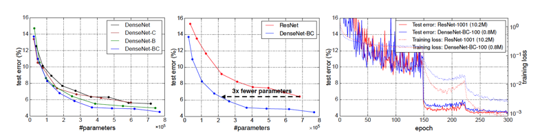
在CIFAR和SVHN数据集上的结果：

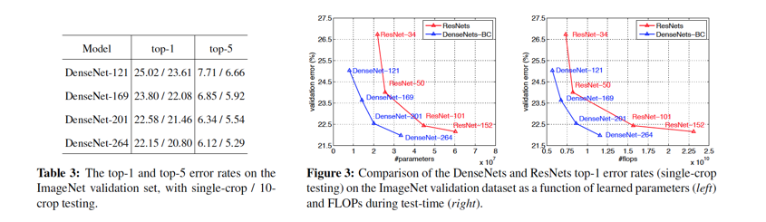
在Imagenet上的结果：

---

文章代码来自：https://github.com/WangXiaoCao/attention-is-all-you-need-pytorch