前言
上一章学习了用逻辑回归函数对MNIST数据集分类,本章将是逻辑回归模型的升级——多层感知器(MLP,神经网络)。本章将学习具有一个隐层的神经网络,它首先将输入进行非线性变换,再输入逻辑回归模型,这样模型就可以拟合非线性问题。非线性层称为隐层,通常一个隐层就可使得模型性能足够优异,但在深度学习中会有更多的隐层。有关神经网络反向梯度更新的理解可以参考:11行Python代码编写神经网络。
MLP模型
具有单隐层的神经网络结构如下图所示:
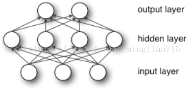
网络对应的映射函数f:Rd->RL,其中d是输入层(input layer)的节点数,L是输出层(output layer)的节点数。f(x)定义:

以上参数:W(1),W(2)为2层的权重系数,b(1),b(2)为偏移系数,s和G为2层的激活函数。
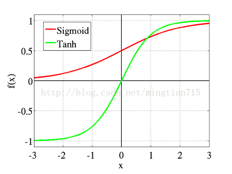
h(x) = s(b(1)+w(1)x)表示隐层节点值,s通常为sigmoid函数,sigmoid(a) = 1/(1+exp(-a)),但此处我们采用激活函数tanh(a) = (exp(a) - exp(-a))/(exp(a) + exp(-a)),因为tanh会使得训练速度更快。tanh函数和sigmoid函数图如下,它们的取值区间不同,但都属于一种压缩函数,且导数形式简单。
o(x)=G(b(2)+W(2)h(x))就是上一章逻辑回归的内容啦,因此激活函数G选择softmax函数。
优化过程依然采用批量梯度下降法,需要确定的参数包括{W(1),W(2),b(1),b(2)},至于如何根据输出更新参数,可以参看我之前有关神经网络的文章。
从逻辑回归到MLP
我们已经有了逻辑回归类了,只需要再定义隐层类:
class HiddenLayer(object):
    def __init__(self, rng, input, n_in, n_out, W=None, b=None,
                 activation=T.tanh):
        """
        Typical hidden layer of a MLP: units are fully-connected and have
        sigmoidal activation function. Weight matrix W is of shape (n_in,n_out)
        and the bias vector b is of shape (n_out,).

        NOTE : The nonlinearity used here is tanh

        Hidden unit activation is given by: tanh(dot(input,W) + b)

        :type rng: numpy.random.RandomState
        :param rng: a random number generator used to initialize weights

        :type input: theano.tensor.dmatrix
        :param input: a symbolic tensor of shape (n_examples, n_in)

        :type n_in: int
        :param n_in: dimensionality of input

        :type n_out: int
        :param n_out: number of hidden units

        :type activation: theano.Op or function
        :param activation: Non linearity to be applied in the hidden
                           layer
        """
        self.input = input
如何初始化隐层权重与激活函数的选择有关,一般是从一个对称区间内随机采样。
激活函数为tanh时,W从![[-\sqrt{\frac{6}{fan_{in}+fan_{out}}},\sqrt{\frac{6}{fan_{in}+fan_{out}}}]](http://www.deeplearning.net/tutorial/_images/math/1dfc4a270526d7a1f3411a25a81a580f05b61d84.png) 采样;激活函数是sigmoid时,从
采样;激活函数是sigmoid时,从![[-4\sqrt{\frac{6}{fan_{in}+fan_{out}}},4\sqrt{\frac{6}{fan_{in}+fan_{out}}}]](http://www.deeplearning.net/tutorial/_images/math/67fb8dc5b0626d0673435da43542cab7e3453c38.png) 采样,其中
采样,其中 是第 i-1 层神经元数量,
 是第 i 层神经元的数量;b初值为0。
采样;激活函数是sigmoid时,从采样,其中是第 i-1 层神经元数量,是第 i 层神经元的数量;b初值为0。
这样初始化可以保证在初始优化阶段,神经网络可以顺利地进行正向传播和反向传播,其实这跟W的梯度公式也有关系,如果W为0,则梯度会一直保持0,网络无法更新。
 # `W` is initialized with `W_values` which is uniformely sampled
        # from sqrt(-6./(n_in+n_hidden)) and sqrt(6./(n_in+n_hidden))
        # for tanh activation function
        # the output of uniform if converted using asarray to dtype
        # theano.config.floatX so that the code is runable on GPU
        # Note : optimal initialization of weights is dependent on the
        #        activation function used (among other things).
        #        For example, results presented in [Xavier10] suggest that you
        #        should use 4 times larger initial weights for sigmoid
        #        compared to tanh
        #        We have no info for other function, so we use the same as
        #        tanh.
        if W is None:
            W_values = numpy.asarray(
                rng.uniform(
                    low=-numpy.sqrt(6. / (n_in + n_out)),
                    high=numpy.sqrt(6. / (n_in + n_out)),
                    size=(n_in, n_out)
                ),
                dtype=theano.config.floatX
            )
            if activation == theano.tensor.nnet.sigmoid:
                W_values *= 4

            W = theano.shared(value=W_values, name='W', borrow=True)

        if b is None:
            b_values = numpy.zeros((n_out,), dtype=theano.config.floatX)
            b = theano.shared(value=b_values, name='b', borrow=True)

        self.W = W
        self.b = b
输出函数如下,默认激活函数为tanh,当然你也可以选择自己希望的。
      lin_output = T.dot(input, self.W) + self.b
        self.output = (
            lin_output if activation is None
            else activation(lin_output)
        )
MLP就是隐层类+逻辑回归类,因此将它们合起来就是MLP,需要定义每一层输入输出,激活函数。其实可以对比一下,隐层类和逻辑回归类很像,不同点主要在于激活函数不同,此外逻辑回归的输出是输出层,因此其输出结果还要用来计算损失函数以及错误率。
class MLP(object):
    """Multi-Layer Perceptron Class

    A multilayer perceptron is a feedforward artificial neural network model
    that has one layer or more of hidden units and nonlinear activations.
    Intermediate layers usually have as activation function tanh or the
    sigmoid function (defined here by a ``HiddenLayer`` class)  while the
    top layer is a softmax layer (defined here by a ``LogisticRegression``
    class).
    """

    def __init__(self, rng, input, n_in, n_hidden, n_out):
        """Initialize the parameters for the multilayer perceptron

        :type rng: numpy.random.RandomState
        :param rng: a random number generator used to initialize weights

        :type input: theano.tensor.TensorType
        :param input: symbolic variable that describes the input of the
        architecture (one minibatch)

        :type n_in: int
        :param n_in: number of input units, the dimension of the space in
        which the datapoints lie

        :type n_hidden: int
        :param n_hidden: number of hidden units

        :type n_out: int
        :param n_out: number of output units, the dimension of the space in
        which the labels lie

        """

        # Since we are dealing with a one hidden layer MLP, this will translate
        # into a HiddenLayer with a tanh activation function connected to the
        # LogisticRegression layer; the activation function can be replaced by
        # sigmoid or any other nonlinear function
        self.hiddenLayer = HiddenLayer(
            rng=rng,
            input=input,
            n_in=n_in,
            n_out=n_hidden,
            activation=T.tanh
        )

        # The logistic regression layer gets as input the hidden units
        # of the hidden layer
        self.logRegressionLayer = LogisticRegression(
            input=self.hiddenLayer.output,
            n_in=n_hidden,
            n_out=n_out
        )
在上一章讲过,为了防止过拟合,会加入正则化项。因此MLP的代价函数就是逻辑回归模型的NLL计算结果再加上正则化项(两层网络权重系数的L1,L2范数)。下面两段代码是程序核心(
代价函数形式和
梯度更新):
       # L1 norm ; one regularization option is to enforce L1 norm to
        # be small
        self.L1 = (
            abs(self.hiddenLayer.W).sum()
            + abs(self.logRegressionLayer.W).sum()
        )

        # square of L2 norm ; one regularization option is to enforce
        # square of L2 norm to be small
        self.L2_sqr = (
            (self.hiddenLayer.W ** 2).sum()
            + (self.logRegressionLayer.W ** 2).sum()
        )

        # negative log likelihood of the MLP is given by the negative
        # log likelihood of the output of the model, computed in the
        # logistic regression layer
        self.negative_log_likelihood = (
            self.logRegressionLayer.negative_log_likelihood
        )
        # same holds for the function computing the number of errors
        self.errors = self.logRegressionLayer.errors

        # the parameters of the model are the parameters of the two layer it is
        # made out of
        self.params = self.hiddenLayer.params + self.logRegressionLayer.params

        # the cost we minimize during training is the negative log likelihood of
    # the model plus the regularization terms (L1 and L2); cost is expressed
    # here symbolically
    cost = (
        classifier.negative_log_likelihood(y)
        + L1_reg * classifier.L1
        + L2_reg * classifier.L2_sqr
    )
最后就是更新网络系数了,Theano采用自己的自动求导方式,输入要求导的项即可。updates 中,前一项是待更新内容,后一项是更新内容。
假设A=[a1,a2,a3],B=[b1,b2,b3],zip(A,B) =[(a1,b1),(a2,b2),(a3,b3)],即可通过遍历zip产生的序列进行逐项更新:
    # compute the gradient of cost with respect to theta (sorted in params)
    # the resulting gradients will be stored in a list gparams
    gparams = [T.grad(cost, param) for param in classifier.params]

    # specify how to update the parameters of the model as a list of
    # (variable, update expression) pairs

    # given two lists of the same length, A = [a1, a2, a3, a4] and
    # B = [b1, b2, b3, b4], zip generates a list C of same size, where each
    # element is a pair formed from the two lists :
    #    C = [(a1, b1), (a2, b2), (a3, b3), (a4, b4)]
    updates = [
        (param, param - learning_rate * gparam)
        for param, gparam in zip(classifier.params, gparams)
    ]

    # compiling a Theano function `train_model` that returns the cost, but
    # in the same time updates the parameter of the model based on the rules
    # defined in `updates`
    train_model = theano.function(
        inputs=[index],
        outputs=cost,
        updates=updates,
        givens={
            x: train_set_x[index * batch_size: (index + 1) * batch_size],
            y: train_set_y[index * batch_size: (index + 1) * batch_size]
        }
    )
train_model函数的输出就是代价函数值(损失函数值)啦。
运行结果
为了运行速度更快,我将学习速率设为0.05,并且将epoch(遍历数据次数,不是优化次数)设为100。由于优化次数少,为了不使代价函数波动过大,将batch_size选为64,结果如下图:
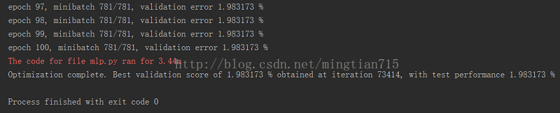
可以对比一下,上一章使用逻辑回归的错误率为7.5%,而此处错误率为1.98%,大幅下降。当然训练时间长达3.44分钟,逻辑回归仅为14s。
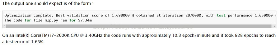
下图为官网教程给出的运行结果,虽然错误率达到了1.65%,但是花费了97分钟。
MLP小技巧
1.tanh相比sigmoid有着更好的收敛性。
2.权重系数初始化,上面已经提及了。
3.学习速率的选择很重要。最简单的方法是恒定学习速率,通过网格搜索(0.01,0.1,1,10...)选择一个最佳学习率使得交叉验证结果最好。另一种方法就是随时间降低学习速率。
4.隐层节点数,越多训练效果越好,也会越慢。
5.正则化系数(常用0.01,0.001..)。
更详细内容:Multilayer Perceptron
如果这篇文章对你有帮助,可以点个赞或者关注我,我会更有动力分享学习过程,谢啦~
完整代码:
"""
This tutorial introduces the multilayer perceptron using Theano.

 A multilayer perceptron is a logistic regressor where
instead of feeding the input to the logistic regression you insert a
intermediate layer, called the hidden layer, that has a nonlinear
activation function (usually tanh or sigmoid) . One can use many such
hidden layers making the architecture deep. The tutorial will also tackle
the problem of MNIST digit classification.

.. math::

    f(x) = G( b^{(2)} + W^{(2)}( s( b^{(1)} + W^{(1)} x))),

References:

    - textbooks: "Pattern Recognition and Machine Learning" -
                 Christopher M. Bishop, section 5

"""

from __future__ import print_function

__docformat__ = 'restructedtext en'


import os
import sys
import timeit

import numpy

import theano
import theano.tensor as T


from logistic_sgd import LogisticRegression, load_data


# start-snippet-1
class HiddenLayer(object):
    def __init__(self, rng, input, n_in, n_out, W=None, b=None,
                 activation=T.tanh):
        """
        Typical hidden layer of a MLP: units are fully-connected and have
        sigmoidal activation function. Weight matrix W is of shape (n_in,n_out)
        and the bias vector b is of shape (n_out,).

        NOTE : The nonlinearity used here is tanh

        Hidden unit activation is given by: tanh(dot(input,W) + b)

        :type rng: numpy.random.RandomState
        :param rng: a random number generator used to initialize weights

        :type input: theano.tensor.dmatrix
        :param input: a symbolic tensor of shape (n_examples, n_in)

        :type n_in: int
        :param n_in: dimensionality of input

        :type n_out: int
        :param n_out: number of hidden units

        :type activation: theano.Op or function
        :param activation: Non linearity to be applied in the hidden
                           layer
        """
        self.input = input
        # end-snippet-1

        # `W` is initialized with `W_values` which is uniformely sampled
        # from sqrt(-6./(n_in+n_hidden)) and sqrt(6./(n_in+n_hidden))
        # for tanh activation function
        # the output of uniform if converted using asarray to dtype
        # theano.config.floatX so that the code is runable on GPU
        # Note : optimal initialization of weights is dependent on the
        #        activation function used (among other things).
        #        For example, results presented in [Xavier10] suggest that you
        #        should use 4 times larger initial weights for sigmoid
        #        compared to tanh
        #        We have no info for other function, so we use the same as
        #        tanh.
        if W is None:
            W_values = numpy.asarray(
                rng.uniform(
                    low=-numpy.sqrt(6. / (n_in + n_out)),
                    high=numpy.sqrt(6. / (n_in + n_out)),
                    size=(n_in, n_out)
                ),
                dtype=theano.config.floatX
            )
            if activation == theano.tensor.nnet.sigmoid:
                W_values *= 4

            W = theano.shared(value=W_values, name='W', borrow=True)

        if b is None:
            b_values = numpy.zeros((n_out,), dtype=theano.config.floatX)
            b = theano.shared(value=b_values, name='b', borrow=True)

        self.W = W
        self.b = b

        lin_output = T.dot(input, self.W) + self.b
        self.output = (
            lin_output if activation is None
            else activation(lin_output)
        )
        # parameters of the model
        self.params = [self.W, self.b]


# start-snippet-2
class MLP(object):
    """Multi-Layer Perceptron Class

    A multilayer perceptron is a feedforward artificial neural network model
    that has one layer or more of hidden units and nonlinear activations.
    Intermediate layers usually have as activation function tanh or the
    sigmoid function (defined here by a ``HiddenLayer`` class)  while the
    top layer is a softmax layer (defined here by a ``LogisticRegression``
    class).
    """

    def __init__(self, rng, input, n_in, n_hidden, n_out):
        """Initialize the parameters for the multilayer perceptron

        :type rng: numpy.random.RandomState
        :param rng: a random number generator used to initialize weights

        :type input: theano.tensor.TensorType
        :param input: symbolic variable that describes the input of the
        architecture (one minibatch)

        :type n_in: int
        :param n_in: number of input units, the dimension of the space in
        which the datapoints lie

        :type n_hidden: int
        :param n_hidden: number of hidden units

        :type n_out: int
        :param n_out: number of output units, the dimension of the space in
        which the labels lie

        """

        # Since we are dealing with a one hidden layer MLP, this will translate
        # into a HiddenLayer with a tanh activation function connected to the
        # LogisticRegression layer; the activation function can be replaced by
        # sigmoid or any other nonlinear function
        self.hiddenLayer = HiddenLayer(
            rng=rng,
            input=input,
            n_in=n_in,
            n_out=n_hidden,
            activation=T.tanh
        )

        # The logistic regression layer gets as input the hidden units
        # of the hidden layer
        self.logRegressionLayer = LogisticRegression(
            input=self.hiddenLayer.output,
            n_in=n_hidden,
            n_out=n_out
        )
        # end-snippet-2 start-snippet-3
        # L1 norm ; one regularization option is to enforce L1 norm to
        # be small
        self.L1 = (
            abs(self.hiddenLayer.W).sum()
            + abs(self.logRegressionLayer.W).sum()
        )

        # square of L2 norm ; one regularization option is to enforce
        # square of L2 norm to be small
        self.L2_sqr = (
            (self.hiddenLayer.W ** 2).sum()
            + (self.logRegressionLayer.W ** 2).sum()
        )

        # negative log likelihood of the MLP is given by the negative
        # log likelihood of the output of the model, computed in the
        # logistic regression layer
        self.negative_log_likelihood = (
            self.logRegressionLayer.negative_log_likelihood
        )
        # same holds for the function computing the number of errors
        self.errors = self.logRegressionLayer.errors

        # the parameters of the model are the parameters of the two layer it is
        # made out of
        self.params = self.hiddenLayer.params + self.logRegressionLayer.params
        # end-snippet-3

        # keep track of model input
        self.input = input


def test_mlp(learning_rate=0.01, L1_reg=0.00, L2_reg=0.0001, n_epochs=1000,
             dataset='mnist.pkl.gz', batch_size=20, n_hidden=500):
    """
    Demonstrate stochastic gradient descent optimization for a multilayer
    perceptron

    This is demonstrated on MNIST.

    :type learning_rate: float
    :param learning_rate: learning rate used (factor for the stochastic
    gradient

    :type L1_reg: float
    :param L1_reg: L1-norm's weight when added to the cost (see
    regularization)

    :type L2_reg: float
    :param L2_reg: L2-norm's weight when added to the cost (see
    regularization)

    :type n_epochs: int
    :param n_epochs: maximal number of epochs to run the optimizer

    :type dataset: string
    :param dataset: the path of the MNIST dataset file from
                 http://www.iro.umontreal.ca/~lisa/deep/data/mnist/mnist.pkl.gz


   """
    datasets = load_data(dataset)

    train_set_x, train_set_y = datasets[0]
    valid_set_x, valid_set_y = datasets[1]
    test_set_x, test_set_y = datasets[2]

    # compute number of minibatches for training, validation and testing
    n_train_batches = train_set_x.get_value(borrow=True).shape[0] // batch_size
    n_valid_batches = valid_set_x.get_value(borrow=True).shape[0] // batch_size
    n_test_batches = test_set_x.get_value(borrow=True).shape[0] // batch_size

    ######################
    # BUILD ACTUAL MODEL #
    ######################
    print('... building the model')

    # allocate symbolic variables for the data
    index = T.lscalar()  # index to a [mini]batch
    x = T.matrix('x')  # the data is presented as rasterized images
    y = T.ivector('y')  # the labels are presented as 1D vector of
                        # [int] labels

    rng = numpy.random.RandomState(1234)

    # construct the MLP class
    classifier = MLP(
        rng=rng,
        input=x,
        n_in=28 * 28,
        n_hidden=n_hidden,
        n_out=10
    )

    # start-snippet-4
    # the cost we minimize during training is the negative log likelihood of
    # the model plus the regularization terms (L1 and L2); cost is expressed
    # here symbolically
    cost = (
        classifier.negative_log_likelihood(y)
        + L1_reg * classifier.L1
        + L2_reg * classifier.L2_sqr
    )
    # end-snippet-4

    # compiling a Theano function that computes the mistakes that are made
    # by the model on a minibatch
    test_model = theano.function(
        inputs=[index],
        outputs=classifier.errors(y),
        givens={
            x: test_set_x[index * batch_size:(index + 1) * batch_size],
            y: test_set_y[index * batch_size:(index + 1) * batch_size]
        }
    )

    validate_model = theano.function(
        inputs=[index],
        outputs=classifier.errors(y),
        givens={
            x: valid_set_x[index * batch_size:(index + 1) * batch_size],
            y: valid_set_y[index * batch_size:(index + 1) * batch_size]
        }
    )

    # start-snippet-5
    # compute the gradient of cost with respect to theta (sorted in params)
    # the resulting gradients will be stored in a list gparams
    gparams = [T.grad(cost, param) for param in classifier.params]

    # specify how to update the parameters of the model as a list of
    # (variable, update expression) pairs

    # given two lists of the same length, A = [a1, a2, a3, a4] and
    # B = [b1, b2, b3, b4], zip generates a list C of same size, where each
    # element is a pair formed from the two lists :
    #    C = [(a1, b1), (a2, b2), (a3, b3), (a4, b4)]
    updates = [
        (param, param - learning_rate * gparam)
        for param, gparam in zip(classifier.params, gparams)
    ]

    # compiling a Theano function `train_model` that returns the cost, but
    # in the same time updates the parameter of the model based on the rules
    # defined in `updates`
    train_model = theano.function(
        inputs=[index],
        outputs=cost,
        updates=updates,
        givens={
            x: train_set_x[index * batch_size: (index + 1) * batch_size],
            y: train_set_y[index * batch_size: (index + 1) * batch_size]
        }
    )
    # end-snippet-5

    ###############
    # TRAIN MODEL #
    ###############
    print('... training')

    # early-stopping parameters
    patience = 10000  # look as this many examples regardless
    patience_increase = 2  # wait this much longer when a new best is
                           # found
    improvement_threshold = 0.995  # a relative improvement of this much is
                                   # considered significant
    validation_frequency = min(n_train_batches, patience // 2)
                                  # go through this many
                                  # minibatche before checking the network
                                  # on the validation set; in this case we
                                  # check every epoch

    best_validation_loss = numpy.inf
    best_iter = 0
    test_score = 0.
    start_time = timeit.default_timer()

    epoch = 0
    done_looping = False

    while (epoch < n_epochs) and (not done_looping):
        epoch = epoch + 1
        for minibatch_index in range(n_train_batches):

            minibatch_avg_cost = train_model(minibatch_index)
            # iteration number
            iter = (epoch - 1) * n_train_batches + minibatch_index

            if (iter + 1) % validation_frequency == 0:
                # compute zero-one loss on validation set
                validation_losses = [validate_model(i) for i
                                     in range(n_valid_batches)]
                this_validation_loss = numpy.mean(validation_losses)

                print(
                    'epoch %i, minibatch %i/%i, validation error %f %%' %
                    (
                        epoch,
                        minibatch_index + 1,
                        n_train_batches,
                        this_validation_loss * 100.
                    )
                )

                # if we got the best validation score until now
                if this_validation_loss < best_validation_loss:
                    #improve patience if loss improvement is good enough
                    if (
                        this_validation_loss < best_validation_loss *
                        improvement_threshold
                    ):
                        patience = max(patience, iter * patience_increase)

                    best_validation_loss = this_validation_loss
                    best_iter = iter

                    # test it on the test set
                    test_losses = [test_model(i) for i
                                   in range(n_test_batches)]
                    test_score = numpy.mean(test_losses)

                    print(('     epoch %i, minibatch %i/%i, test error of '
                           'best model %f %%') %
                          (epoch, minibatch_index + 1, n_train_batches,
                           test_score * 100.))

            if patience <= iter:
                done_looping = True
                break

    end_time = timeit.default_timer()
    print(('Optimization complete. Best validation score of %f %% '
           'obtained at iteration %i, with test performance %f %%') %
          (best_validation_loss * 100., best_iter + 1, test_score * 100.))
    print(('The code for file ' +
           os.path.split(__file__)[1] +
           ' ran for %.2fm' % ((end_time - start_time) / 60.)), file=sys.stderr)


if __name__ == '__main__':
    test_mlp()